Numerical simulations - Limited area model

To support the campaign, we performed daily hindcasts of the atmospheric conditions in the campaign region. The whole dataset is catalogued and stored on the supercomputer Levante, hosted by the DKRZ and is accessible on demand. It comprises of high-sampling rate 2D and 3D snapshots of key variables.

Visualisations of individual variables for each day are given here. A sample script showing how to load and plot the data is provided below.

Requires zarr>=3

The dataset is stored in Zarr v3 and thus requires zarr>=3.0.0.

Matplotlib style sheet

This script makes use of a custom Matplotlib style sheet: dark.mplstyle

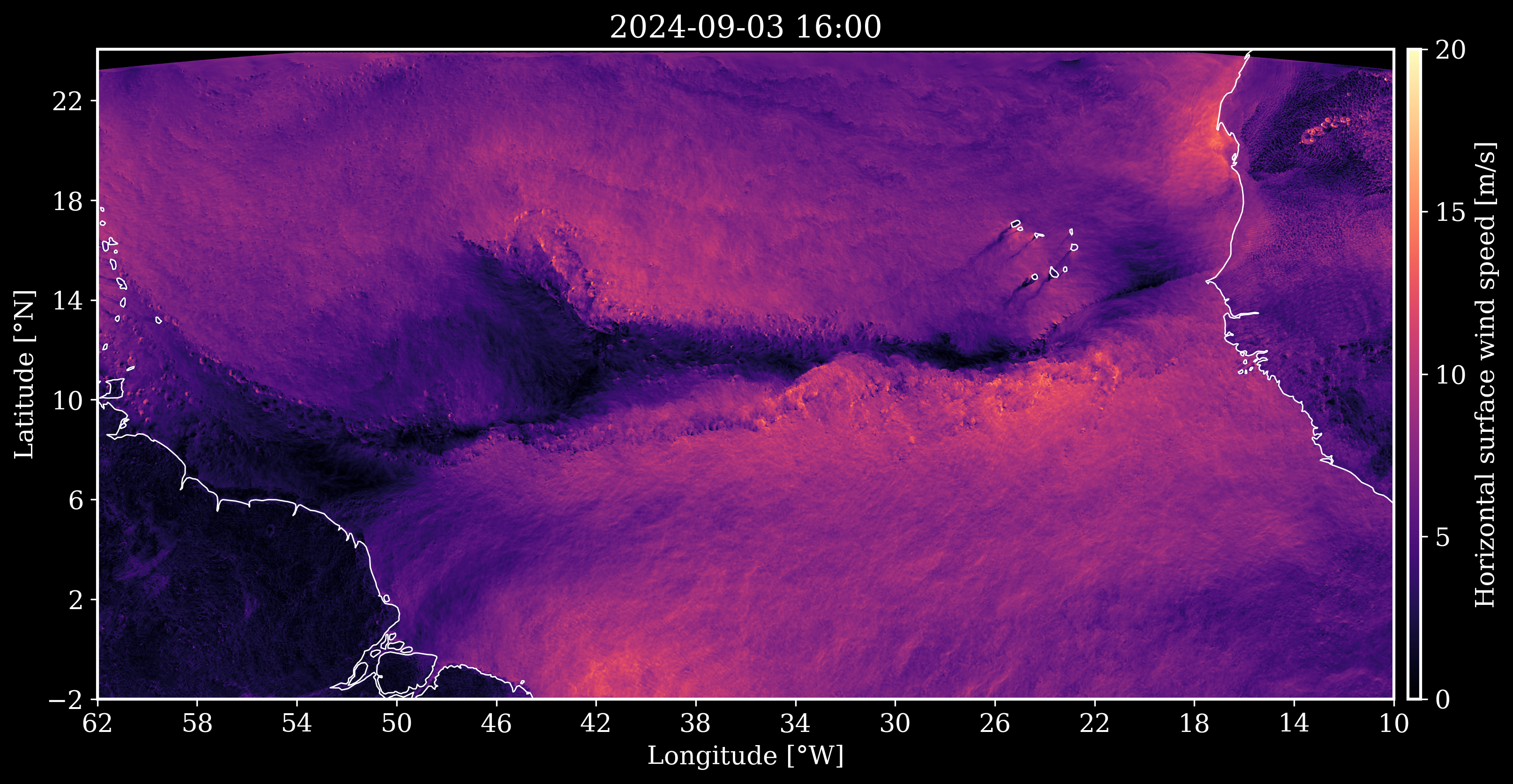
This script shows how to read the LAM-ORCESTRA HEALPix dataset. It plots a contour of horizontal surface wind speed for a specific time.

import cartopy.crs as ccrs
import easygems.healpix as egh
import intake
import matplotlib.pyplot as plt
import numpy as np
import xarray as xr
from mpl_toolkits.axes_grid1 import make_axes_locatable


# Apply custom dark background style
plt.style.use("./dark.mplstyle")


def apply_figure_style(ax, fig):
    """Black background style for figures."""
    ax.set_extent([-62, -10, -2, 22])
    ax.coastlines(color="white", linewidth=0.7)
    ax.set_xlabel("Longitude [°W]")
    ax.set_xticks(np.linspace(-62, -10, 14), crs=ccrs.PlateCarree())
    ax.xaxis.set_major_formatter(plt.FuncFormatter(lambda x, pos: f"{abs(int(x))}"))
    ax.set_ylabel("Latitude [°N]")
    ax.set_yticks(np.linspace(-2, 22, 7), crs=ccrs.PlateCarree())


# Open the 2d dataset spanning the full-campaign period
url = "https://eerie.cloud.dkrz.de/datasets/orcestra_1250m_2d_hpz12/kerchunk"
ds = xr.open_dataset(url, chunks={}, engine="zarr", zarr_format=3)

# Local dataset access (on Levante only!)
# cat = intake.open_catalog("https://tcodata.mpimet.mpg.de/internal.yaml")
# ds = cat.ORCESTRA.LAM_ORCESTRA(dim="2d").to_dask()

# Compute surface wind speed
ds = ds.assign(sfcwind=lambda dx: np.hypot(dx.uas, dx.vas))

# Select and plot horizontal surface wind speed at 16:00h
time = "2024-09-03 16:00"

fig, ax = plt.subplots(figsize=(13, 6), subplot_kw={"projection": ccrs.PlateCarree()})
apply_figure_style(ax, fig)

im = egh.healpix_show(ds.sfcwind.sel(time=time), vmin=0, vmax=20, cmap="magma", ax=ax)

# Add colorbar
cax = make_axes_locatable(ax).append_axes("right", size="1%", pad=0.1, axes_class=plt.Axes)
fig.colorbar(im, cax=cax, ticks=range(0, 21, 5), label="Horizontal surface wind speed [m/s]")

# Add title with formatted timestamp
ax.set_title(time);