
Flight plan docs (Python)#
The orcestra.flightplan module provides a few functions to create flight plans in declarative and constructive style. It is based on defining waypoints and circles, forming a flight path.
Waypoints#
Points (i.e. LatLon objects) can have several attributes, one of them is the label, used to identify the point. Attributes can either be defined when creating the point within the constructor, or assigned later on. Note that assign technically creates a new object and does not modify the old object in place.
The FlightPlan objects assists with computations, analysis and export of the flight plan. For now, just remember to wrap a list of waypoints in a FlightPlan object.
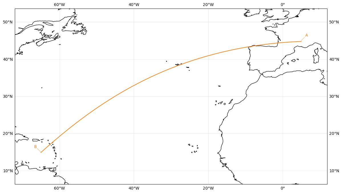
from orcestra.flightplan import LatLon, FlightPlan

plan = FlightPlan([
    LatLon(45, 5, label="A"),
    LatLon(15, -65).assign(label="B"),
])
plan.preview();
Note
The connection between two points will be calculated as a great circle. This is the shortest distance between two points and what aircraft usually fly, but it’s different from how satellites typically fly and it’s also different from a straight line in a lat/lon plot. If you need to stick to a different path, you may want to add additional points in between.
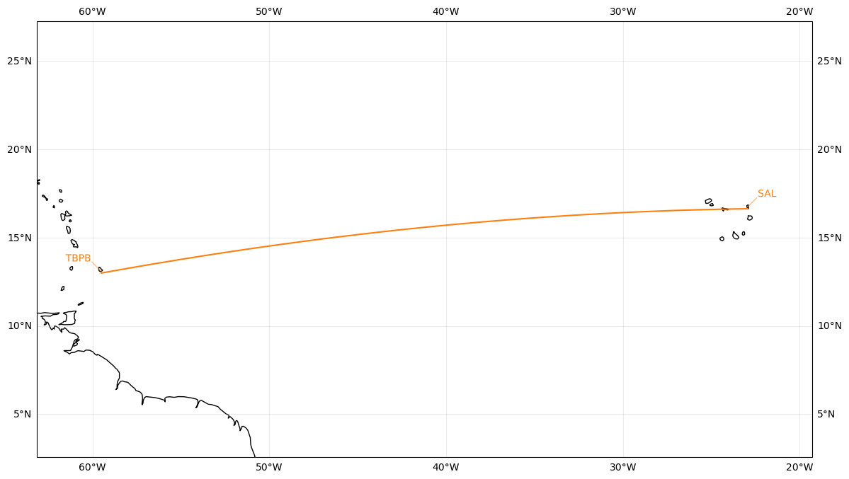
Some commonly used points are predefined, you can import and use them as needed:
from orcestra.flightplan import sal, tbpb

FlightPlan([sal, tbpb]).preview();
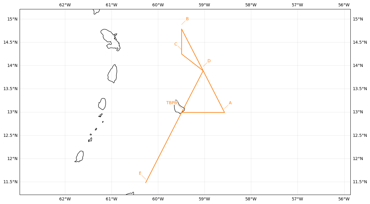
You can construct new points, based on existing points, using the course and towards methods:
A = tbpb.course(90, 100e3).assign(label="A")  # start at 90° from north, move 100km
B = tbpb.course(0, 200e3).assign(label="B")
C = B.towards(tbpb, fraction=.3).assign(label="C")  # start at B, go 30% of the distance towards tbpb
D = B.towards(A).assign(label="D")  # midpoint by default
E = D.towards(tbpb, distance=300e3).assign(label="E")  # you can use absolute distances and even overshoot the target point
FlightPlan([tbpb, A, B, C, D, E]).preview();
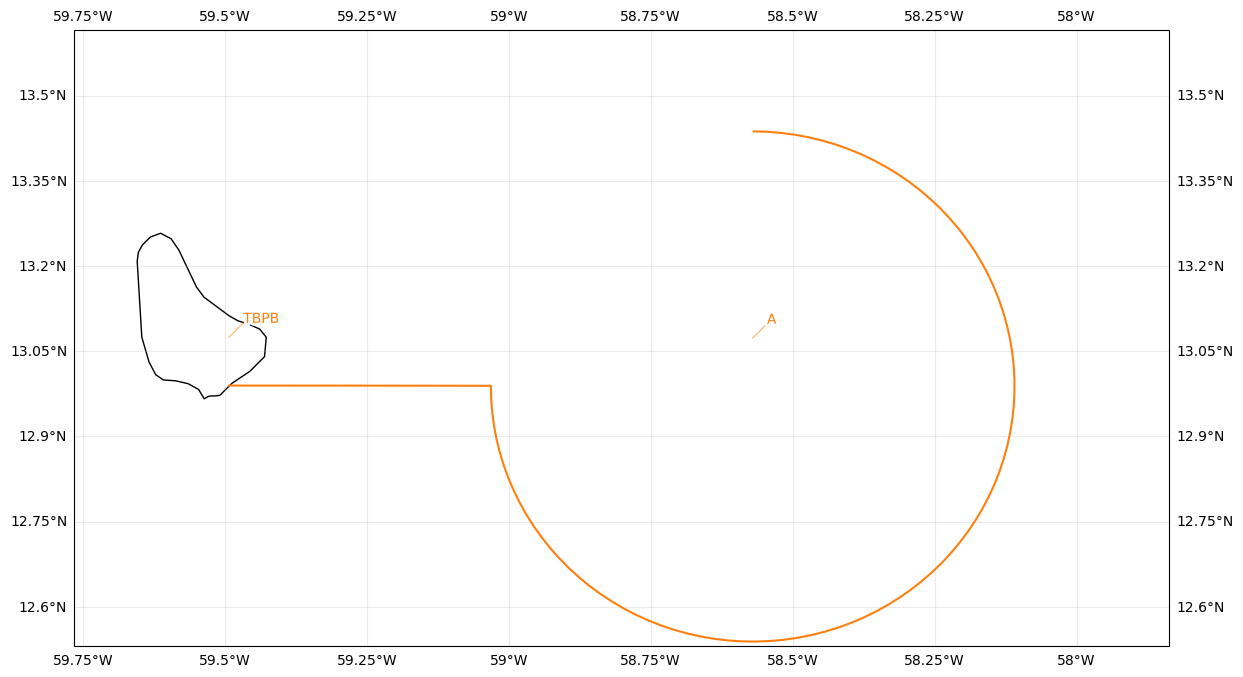
Circles#
In addition to great circle lines, it’s possible to construct circles on the map. The exact orientation of the circle will depend on the previous point, that’s why it’s called IntoCircle:
from orcestra.flightplan import IntoCircle

FlightPlan([
    tbpb,
    IntoCircle(A, radius=50e3, angle=-270)  # 50km radius, 270deg counter clockwise circle
]).preview();
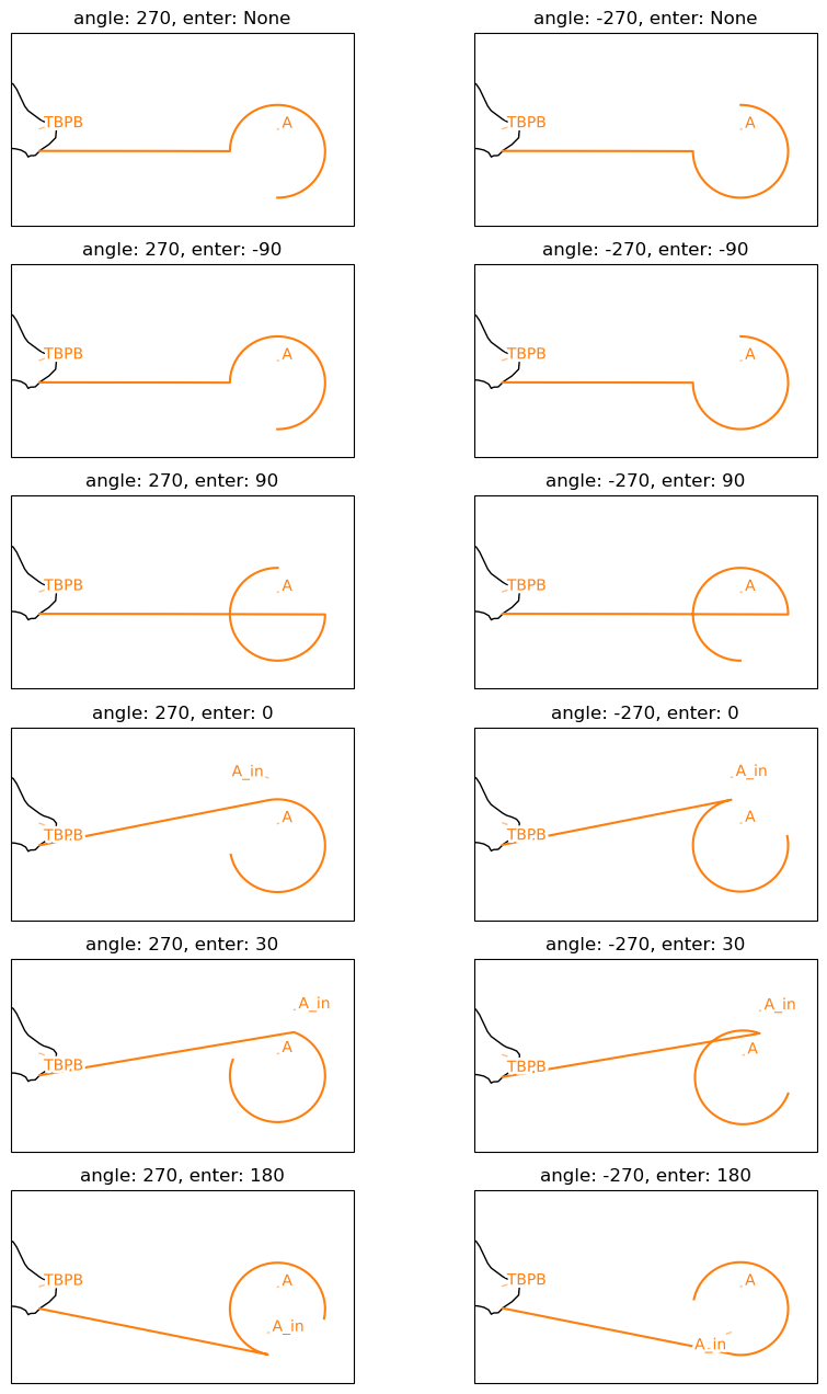
IntoCircle as some arguments which can be used to influence how the circle is computed.
The
angleargument defines the direction and distance to fly along the circle in degrees. Positive values result in a clockwise (CW) flight and negative values in a counter clockwise (CCW) flight.The
enterargument is optional. If given, the circle is entered with a certain turning angle (e.g.enter=-90== enter the circle with a 90° CCW turn). Note that negativeanglevalues mean “start backwards”, which might be confusing first, but ensures thatenterdetermines where to enter the circle andangledetermines the direction and distance.
The coordinate at which the circle will be entered will be computed to match this angle. It’s probably best explained using some pictures, thus, the following plots show several combinations of the angle and enter arguments:
Flight Levels#
In adition to the horizontal track, waypoints can be annotated with flight levels to add a vertical component to the flight track.
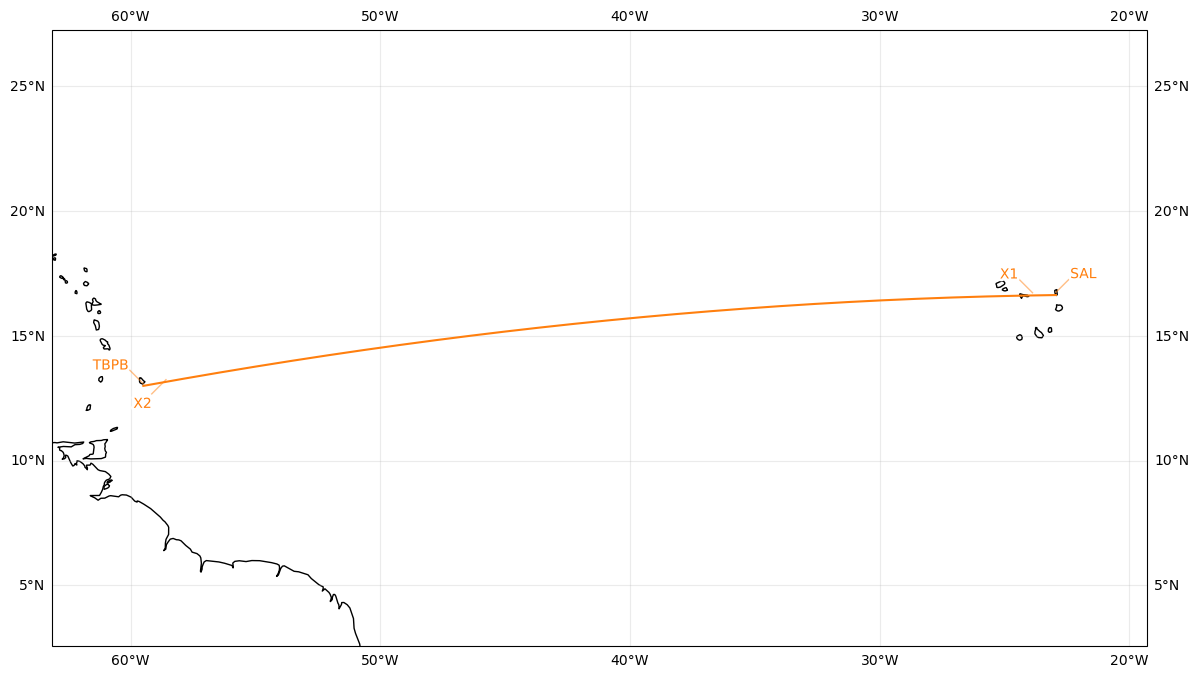
X1 = sal.towards(tbpb, distance=100e3).assign(label="X1", fl=400)
X2 = tbpb.towards(sal, distance=100e3).assign(label="X2", fl=420)
plan = FlightPlan([sal, X1, X2, tbpb])
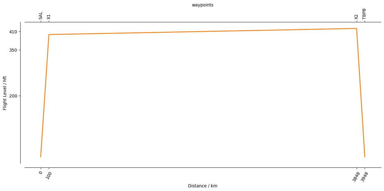
plan.preview();
plan.profile();
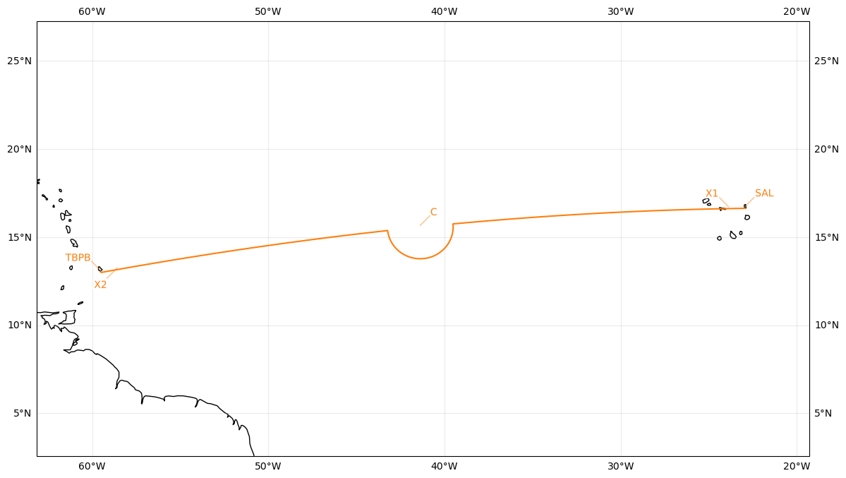
You can also assign flight levels to the center coordinate of a circle. In that case, the whole circle will be flown at that altitude:
plan = FlightPlan([
    sal, X1,
    IntoCircle(X1.towards(X2).assign(fl=450, label="C"), radius=200e3, angle=180),
    X2, tbpb
])
plan.preview();plan.profile();

Aircraft Performance#
If the flight plan contains flight level annotations, it’s possible to use aircraft performance data to compute durations and times along the flight path. In order to load the right flight performance data, you should specify the aircraft within the FlightPlan:
plan = FlightPlan([sal, X1, X2, tbpb], aircraft="HALO")
print(plan.duration)
4:43:33.195870
You may annotate any one of the waypoints with a time. If you do so, each step along the flight path will get a computed time. This also sets takeoff_time and landing_time:
plan = FlightPlan(
    [sal.assign(time="2024-09-06T10:00Z"), X1, X2, tbpb],
    aircraft="HALO")
print("takeoff", plan.takeoff_time)
print("landing", plan.landing_time)
print("duration", plan.duration)
takeoff 2024-09-06 10:00:00+00:00
landing 2024-09-06 14:43:33.195870+00:00
duration 4:43:33.195870
plan = FlightPlan(
    [sal, X1, X2.assign(time="2024-09-06T10:00Z"), tbpb],
    aircraft="HALO")
print("takeoff", plan.takeoff_time)
print("landing", plan.landing_time)
print("duration", plan.duration)
takeoff 2024-09-06 05:24:54.662222+00:00
landing 2024-09-06 10:08:27.858093+00:00
duration 4:43:33.195870
Export#
You can export the flight plan into various formats. First, there’s a short textual view, which can be printed using show_details():
plan.show_details()
Detailed Overview:
              SAL          N16 44.07, W022 56.64, FL000, 05:24:54 UTC,
to            X1           N16 43.17, W023 52.90, FL400, 05:33:26 UTC,
to            X2           N13 14.30, W058 35.12, FL420, 10:00:00 UTC,
to            TBPB         N13 04.48, W059 29.55, FL000, 10:08:27 UTC,
There’s also a generic export() function, which presents multiple formats as download-buttons. In order to use that (and also in general), you have to specify a flight_id for the FlightPlan, and you should also specify a crew:
plan = FlightPlan(
    [
        sal, X1,
        IntoCircle(X1.towards(X2).assign(fl=450, label="C"), radius=200e3, angle=180),
        X2, tbpb.assign(time="2024-09-06T20:00Z")
    ],
    flight_id="DEMO-01",
    aircraft="HALO",
    crew={"Observer": "John Doe"},
)
plan.export()