
ERA5 data on the HEALPix grid#
ERA5[1] data for selected variables has been restructured and remapped onto the HEALPix grid for the years 2010 to 2023. This dataset, which we call HERA5, is accessible through the internal TCO catalog and can be read and used by everyone. HERA5 provides data at different temporal resolutions and enables an open and fast access to the data from everywhere and without a local copy. This notebook shows the access to the data and some basic usage examples.
This tutorial makes use of the easygems python package which hosts several convenience functions to work with and display Earth-system data on the HEALPix grid.
If you don’t have the package installed, you can run the code cell below to install it via pip:
%pip install easygems
Loading the data from the catalog#
First, let’s import all packages that are required to run the full notebook.
import intake
import healpix as hp
import cmocean
import numpy as np
import xarray as xr

import cartopy.crs as ccrs
import cartopy.feature as cf
import matplotlib.pyplot as plt

import easygems.healpix as egh
Now we can open the catalog and select the hierarchical HEALPix ERA5 data HERA5.
cat = intake.open_catalog("https://tcodata.mpimet.mpg.de/internal.yaml")
list(cat)
['BCO', 'METEOR', 'ORCESTRA', 'HERA5', 'HIFS', 'airinfo']
cat.HERA5.to_dask().pipe(egh.attach_coords)
/home/runner/miniconda3/envs/orcestra_book/lib/python3.12/site-packages/intake_xarray/xzarr.py:44: FutureWarning: In a future version of xarray the default value for compat will change from compat='no_conflicts' to compat='override'. This is likely to lead to different results when combining overlapping variables with the same name. To opt in to new defaults and get rid of these warnings now use `set_options(use_new_combine_kwarg_defaults=True) or set compat explicitly.
  self._ds = xr.open_mfdataset(self.urlpath, **kw)
/home/runner/miniconda3/envs/orcestra_book/lib/python3.12/site-packages/intake_xarray/base.py:21: FutureWarning: The return type of `Dataset.dims` will be changed to return a set of dimension names in future, in order to be more consistent with `DataArray.dims`. To access a mapping from dimension names to lengths, please use `Dataset.sizes`.
  'dims': dict(self._ds.dims),
<xarray.Dataset> Size: 66GB
Dimensions:    (time: 164, cell: 196608, level: 29)
Coordinates:
  * time       (time) datetime64[ns] 1kB 2010-01-16T04:15:00 ... 2023-08-16T0...
  * cell       (cell) int64 2MB 0 1 2 3 4 ... 196603 196604 196605 196606 196607
    latitude   (cell) float32 786kB dask.array<chunksize=(196608,), meta=np.ndarray>
    longitude  (cell) float32 786kB dask.array<chunksize=(196608,), meta=np.ndarray>
    lat        (cell) float64 2MB 0.2984 0.5968 0.5968 ... -0.5968 -0.2984
    lon        (cell) float64 2MB 45.0 45.35 44.65 45.0 ... 315.4 314.6 315.0
  * level      (level) int64 232B 50 70 100 125 150 175 ... 900 925 950 975 1000
    crs        int64 8B 0
Data variables: (12/73)
    100u       (time, cell) float32 129MB dask.array<chunksize=(24, 4096), meta=np.ndarray>
    100v       (time, cell) float32 129MB dask.array<chunksize=(24, 4096), meta=np.ndarray>
    10si       (time, cell) float32 129MB dask.array<chunksize=(24, 4096), meta=np.ndarray>
    10u        (time, cell) float32 129MB dask.array<chunksize=(24, 4096), meta=np.ndarray>
    10v        (time, cell) float32 129MB dask.array<chunksize=(24, 4096), meta=np.ndarray>
    2d         (time, cell) float32 129MB dask.array<chunksize=(24, 4096), meta=np.ndarray>
    ...         ...
    isor       (cell) float32 786kB dask.array<chunksize=(196608,), meta=np.ndarray>
    lsm        (cell) float32 786kB dask.array<chunksize=(196608,), meta=np.ndarray>
    sdfor      (cell) float32 786kB dask.array<chunksize=(196608,), meta=np.ndarray>
    sdor       (cell) float32 786kB dask.array<chunksize=(196608,), meta=np.ndarray>
    slor       (cell) float32 786kB dask.array<chunksize=(196608,), meta=np.ndarray>
    z_sfc      (cell) float32 786kB dask.array<chunksize=(196608,), meta=np.ndarray>
Attributes:
    title:           HERA5 - HEALPixelation of ERA5
    description:     Selected variables from ERA5, restructured and saved on ...
    source:          Post-processed dataset based on the ERA5 mirror located ...
    creator:         Lukas Kluft
    institution:     Max Planck Institute for Meteorology
    contact:         lukas.kluft@mpimet.mpg.de
acknowledgment: Contains modified Copernicus Climate Change Service info...- time: 164
- cell: 196608
- level: 29
- time(time)datetime64[ns]2010-01-16T04:15:00 ... 2023-08-...
- axis :
- T
array(['2010-01-16T04:15:00.000000000', '2010-02-16T04:15:00.000000000', '2010-03-16T04:15:00.000000000', '2010-04-16T03:15:00.000000000', '2010-05-16T03:15:00.000000000', '2010-06-16T03:15:00.000000000', '2010-07-16T03:15:00.000000000', '2010-08-16T03:15:00.000000000', '2010-09-16T03:15:00.000000000', '2010-10-16T03:15:00.000000000', '2010-11-16T04:15:00.000000000', '2010-12-16T04:15:00.000000000', '2011-01-16T04:15:00.000000000', '2011-02-16T04:15:00.000000000', '2011-03-16T04:15:00.000000000', '2011-04-16T03:15:00.000000000', '2011-05-16T03:15:00.000000000', '2011-06-16T03:15:00.000000000', '2011-07-16T03:15:00.000000000', '2011-08-16T03:15:00.000000000', '2011-09-16T03:15:00.000000000', '2011-10-16T03:15:00.000000000', '2011-11-16T04:15:00.000000000', '2011-12-16T04:15:00.000000000', '2012-01-16T04:15:00.000000000', '2012-02-16T04:15:00.000000000', '2012-03-16T04:15:00.000000000', '2012-04-16T03:15:00.000000000', '2012-05-16T03:15:00.000000000', '2012-06-16T03:15:00.000000000', '2012-07-16T03:15:00.000000000', '2012-08-16T03:15:00.000000000', '2012-09-16T03:15:00.000000000', '2012-10-16T03:15:00.000000000', '2012-11-16T04:15:00.000000000', '2012-12-16T04:15:00.000000000', '2013-01-16T04:15:00.000000000', '2013-02-16T04:15:00.000000000', '2013-03-16T04:15:00.000000000', '2013-04-16T03:15:00.000000000', '2013-05-16T03:15:00.000000000', '2013-06-16T03:15:00.000000000', '2013-07-16T03:15:00.000000000', '2013-08-16T03:15:00.000000000', '2013-09-16T03:15:00.000000000', '2013-10-16T03:15:00.000000000', '2013-11-16T04:15:00.000000000', '2013-12-16T04:15:00.000000000', '2014-01-16T04:15:00.000000000', '2014-02-16T04:15:00.000000000', '2014-03-16T04:15:00.000000000', '2014-04-16T03:15:00.000000000', '2014-05-16T03:15:00.000000000', '2014-06-16T03:15:00.000000000', '2014-07-16T03:15:00.000000000', '2014-08-16T03:15:00.000000000', '2014-09-16T03:15:00.000000000', '2014-10-16T03:15:00.000000000', '2014-11-16T04:15:00.000000000', '2014-12-16T04:15:00.000000000', '2015-01-16T04:15:00.000000000', '2015-02-16T04:15:00.000000000', '2015-03-16T04:15:00.000000000', '2015-04-16T03:15:00.000000000', '2015-05-16T03:15:00.000000000', '2015-06-16T03:15:00.000000000', '2015-07-16T03:15:00.000000000', '2015-08-16T03:15:00.000000000', '2015-09-16T03:15:00.000000000', '2015-10-16T03:15:00.000000000', '2015-11-16T04:15:00.000000000', '2015-12-16T04:15:00.000000000', '2016-01-16T04:15:00.000000000', '2016-02-16T04:15:00.000000000', '2016-03-16T04:15:00.000000000', '2016-04-16T03:15:00.000000000', '2016-05-16T03:15:00.000000000', '2016-06-16T03:15:00.000000000', '2016-07-16T03:15:00.000000000', '2016-08-16T03:15:00.000000000', '2016-09-16T03:15:00.000000000', '2016-10-16T03:15:00.000000000', '2016-11-16T04:15:00.000000000', '2016-12-16T04:15:00.000000000', '2017-01-16T04:15:00.000000000', '2017-02-16T04:15:00.000000000', '2017-03-16T04:15:00.000000000', '2017-04-16T03:15:00.000000000', '2017-05-16T03:15:00.000000000', '2017-06-16T03:15:00.000000000', '2017-07-16T03:15:00.000000000', '2017-08-16T03:15:00.000000000', '2017-09-16T03:15:00.000000000', '2017-10-16T03:15:00.000000000', '2017-11-16T04:15:00.000000000', '2017-12-16T04:15:00.000000000', '2018-01-16T04:15:00.000000000', '2018-02-16T04:15:00.000000000', '2018-03-16T04:15:00.000000000', '2018-04-16T03:15:00.000000000', '2018-05-16T03:15:00.000000000', '2018-06-16T03:15:00.000000000', '2018-07-16T03:15:00.000000000', '2018-08-16T03:15:00.000000000', '2018-09-16T03:15:00.000000000', '2018-10-16T03:15:00.000000000', '2018-11-16T04:15:00.000000000', '2018-12-16T04:15:00.000000000', '2019-01-16T04:15:00.000000000', '2019-02-16T04:15:00.000000000', '2019-03-16T04:15:00.000000000', '2019-04-16T03:15:00.000000000', '2019-05-16T03:15:00.000000000', '2019-06-16T03:15:00.000000000', '2019-07-16T03:15:00.000000000', '2019-08-16T03:15:00.000000000', '2019-09-16T03:15:00.000000000', '2019-10-16T03:15:00.000000000', '2019-11-16T04:15:00.000000000', '2019-12-16T04:15:00.000000000', '2020-01-16T04:15:00.000000000', '2020-02-16T04:15:00.000000000', '2020-03-16T04:15:00.000000000', '2020-04-16T03:15:00.000000000', '2020-05-16T03:15:00.000000000', '2020-06-16T03:15:00.000000000', '2020-07-16T03:15:00.000000000', '2020-08-16T03:15:00.000000000', '2020-09-16T03:15:00.000000000', '2020-10-16T03:15:00.000000000', '2020-11-16T04:15:00.000000000', '2020-12-16T04:15:00.000000000', '2021-01-16T04:15:00.000000000', '2021-02-16T04:15:00.000000000', '2021-03-16T04:15:00.000000000', '2021-04-16T03:15:00.000000000', '2021-05-16T03:15:00.000000000', '2021-06-16T03:15:00.000000000', '2021-07-16T03:15:00.000000000', '2021-08-16T03:15:00.000000000', '2021-09-16T03:15:00.000000000', '2021-10-16T03:15:00.000000000', '2021-11-16T04:15:00.000000000', '2021-12-16T04:15:00.000000000', '2022-01-16T04:15:00.000000000', '2022-02-16T04:15:00.000000000', '2022-03-16T04:15:00.000000000', '2022-04-16T03:15:00.000000000', '2022-05-16T03:15:00.000000000', '2022-06-16T03:15:00.000000000', '2022-07-16T03:15:00.000000000', '2022-08-16T03:15:00.000000000', '2022-09-16T03:15:00.000000000', '2022-10-16T03:15:00.000000000', '2022-11-16T04:15:00.000000000', '2022-12-16T04:15:00.000000000', '2023-01-16T04:15:00.000000000', '2023-02-16T04:15:00.000000000', '2023-03-16T04:15:00.000000000', '2023-04-16T03:15:00.000000000', '2023-05-16T03:15:00.000000000', '2023-06-16T03:15:00.000000000', '2023-07-16T03:15:00.000000000', '2023-08-16T03:15:00.000000000'], dtype='datetime64[ns]') - cell(cell)int640 1 2 3 ... 196605 196606 196607
- standard_name :
- healpix_index
array([ 0, 1, 2, ..., 196605, 196606, 196607], shape=(196608,))
- latitude(cell)float32dask.array<chunksize=(196608,), meta=np.ndarray>
- long_name :
- latitude
- standard_name :
- latitude
- units :
- degrees_north
Array Chunk Bytes 768.00 kiB 768.00 kiB Shape (196608,) (196608,) Dask graph 1 chunks in 5 graph layers Data type float32 numpy.ndarray - longitude(cell)float32dask.array<chunksize=(196608,), meta=np.ndarray>
- long_name :
- longitude
- standard_name :
- longitude
- units :
- degrees_east
Array Chunk Bytes 768.00 kiB 768.00 kiB Shape (196608,) (196608,) Dask graph 1 chunks in 5 graph layers Data type float32 numpy.ndarray - lat(cell)float640.2984 0.5968 ... -0.5968 -0.2984
- units :
- degree_north
- standard_name :
- latitude
- axis :
- Y
array([ 0.29841687, 0.59684183, 0.59684183, ..., -0.59684183, -0.59684183, -0.29841687], shape=(196608,)) - lon(cell)float6445.0 45.35 44.65 ... 314.6 315.0
- units :
- degree_east
- standard_name :
- longitude
- axis :
- X
array([ 45. , 45.3515625, 44.6484375, ..., 315.3515625, 314.6484375, 315. ], shape=(196608,)) - level(level)int6450 70 100 125 ... 925 950 975 1000
- axis :
- Z
- long_name :
- Air pressure at model level
- positive :
- down
- standard_name :
- air_pressure
- units :
- hPa
array([ 50, 70, 100, 125, 150, 175, 200, 225, 250, 300, 350, 400, 450, 500, 550, 600, 650, 700, 750, 775, 800, 825, 850, 875, 900, 925, 950, 975, 1000]) - crs()int640
- grid_mapping_name :
- healpix
- refinement_level :
- 7
- indexing_scheme :
- nested
array(0)
- 100u(time, cell)float32dask.array<chunksize=(24, 4096), meta=np.ndarray>
- levtype :
- surface
- long_name :
- 100 metre U wind component
- standard_name :
- type :
- analysis
- units :
- m s**-1
Array Chunk Bytes 123.00 MiB 384.00 kiB Shape (164, 196608) (24, 4096) Dask graph 336 chunks in 2 graph layers Data type float32 numpy.ndarray - 100v(time, cell)float32dask.array<chunksize=(24, 4096), meta=np.ndarray>
- levtype :
- surface
- long_name :
- 100 metre V wind component
- standard_name :
- type :
- analysis
- units :
- m s**-1
Array Chunk Bytes 123.00 MiB 384.00 kiB Shape (164, 196608) (24, 4096) Dask graph 336 chunks in 2 graph layers Data type float32 numpy.ndarray - 10si(time, cell)float32dask.array<chunksize=(24, 4096), meta=np.ndarray>
- levtype :
- surface
- long_name :
- 10 metre wind speed
- standard_name :
- units :
- m s**-1
Array Chunk Bytes 123.00 MiB 384.00 kiB Shape (164, 196608) (24, 4096) Dask graph 336 chunks in 2 graph layers Data type float32 numpy.ndarray - 10u(time, cell)float32dask.array<chunksize=(24, 4096), meta=np.ndarray>
- levtype :
- surface
- long_name :
- 10 metre U wind component
- standard_name :
- type :
- analysis
- units :
- m s**-1
Array Chunk Bytes 123.00 MiB 384.00 kiB Shape (164, 196608) (24, 4096) Dask graph 336 chunks in 2 graph layers Data type float32 numpy.ndarray - 10v(time, cell)float32dask.array<chunksize=(24, 4096), meta=np.ndarray>
- levtype :
- surface
- long_name :
- 10 metre V wind component
- standard_name :
- type :
- analysis
- units :
- m s**-1
Array Chunk Bytes 123.00 MiB 384.00 kiB Shape (164, 196608) (24, 4096) Dask graph 336 chunks in 2 graph layers Data type float32 numpy.ndarray - 2d(time, cell)float32dask.array<chunksize=(24, 4096), meta=np.ndarray>
- levtype :
- surface
- long_name :
- 2 metre dewpoint temperature
- standard_name :
- type :
- analysis
- units :
- K
Array Chunk Bytes 123.00 MiB 384.00 kiB Shape (164, 196608) (24, 4096) Dask graph 336 chunks in 2 graph layers Data type float32 numpy.ndarray - 2t(time, cell)float32dask.array<chunksize=(24, 4096), meta=np.ndarray>
- levtype :
- surface
- long_name :
- 2 metre temperature
- standard_name :
- type :
- analysis
- units :
- K
Array Chunk Bytes 123.00 MiB 384.00 kiB Shape (164, 196608) (24, 4096) Dask graph 336 chunks in 2 graph layers Data type float32 numpy.ndarray - asn(time, cell)float32dask.array<chunksize=(24, 4096), meta=np.ndarray>
- levtype :
- surface
- long_name :
- Snow albedo
- standard_name :
- type :
- analysis
- units :
- (0 - 1)
Array Chunk Bytes 123.00 MiB 384.00 kiB Shape (164, 196608) (24, 4096) Dask graph 336 chunks in 2 graph layers Data type float32 numpy.ndarray - blh(time, cell)float32dask.array<chunksize=(24, 4096), meta=np.ndarray>
- levtype :
- surface
- long_name :
- Boundary layer height
- standard_name :
- type :
- forecast
- units :
- m
Array Chunk Bytes 123.00 MiB 384.00 kiB Shape (164, 196608) (24, 4096) Dask graph 336 chunks in 2 graph layers Data type float32 numpy.ndarray - cape(time, cell)float32dask.array<chunksize=(24, 4096), meta=np.ndarray>
- levtype :
- surface
- long_name :
- Convective available potential energy
- standard_name :
- type :
- forecast
- units :
- J kg**-1
Array Chunk Bytes 123.00 MiB 384.00 kiB Shape (164, 196608) (24, 4096) Dask graph 336 chunks in 2 graph layers Data type float32 numpy.ndarray - cbh(time, cell)float32dask.array<chunksize=(24, 4096), meta=np.ndarray>
- levtype :
- surface
- long_name :
- Cloud base height
- standard_name :
- type :
- forecast
- units :
- m
Array Chunk Bytes 123.00 MiB 384.00 kiB Shape (164, 196608) (24, 4096) Dask graph 336 chunks in 2 graph layers Data type float32 numpy.ndarray - cc(time, level, cell)float32dask.array<chunksize=(24, 4, 1024), meta=np.ndarray>
- levtype :
- isobaricInhPa
- long_name :
- Fraction of cloud cover
- standard_name :
- type :
- analysis
- units :
- (0 - 1)
Array Chunk Bytes 3.48 GiB 384.00 kiB Shape (164, 29, 196608) (24, 4, 1024) Dask graph 10752 chunks in 2 graph layers Data type float32 numpy.ndarray - ci(time, cell)float32dask.array<chunksize=(24, 4096), meta=np.ndarray>
- levtype :
- surface
- long_name :
- Sea ice area fraction
- standard_name :
- sea_ice_area_fraction
- type :
- analysis
- units :
- (0 - 1)
Array Chunk Bytes 123.00 MiB 384.00 kiB Shape (164, 196608) (24, 4096) Dask graph 336 chunks in 2 graph layers Data type float32 numpy.ndarray - ciwc(time, level, cell)float32dask.array<chunksize=(24, 4, 1024), meta=np.ndarray>
- levtype :
- isobaricInhPa
- long_name :
- Specific cloud ice water content
- standard_name :
- type :
- analysis
- units :
- kg kg**-1
Array Chunk Bytes 3.48 GiB 384.00 kiB Shape (164, 29, 196608) (24, 4, 1024) Dask graph 10752 chunks in 2 graph layers Data type float32 numpy.ndarray - clwc(time, level, cell)float32dask.array<chunksize=(24, 4, 1024), meta=np.ndarray>
- levtype :
- isobaricInhPa
- long_name :
- Specific cloud liquid water content
- standard_name :
- type :
- analysis
- units :
- kg kg**-1
Array Chunk Bytes 3.48 GiB 384.00 kiB Shape (164, 29, 196608) (24, 4, 1024) Dask graph 10752 chunks in 2 graph layers Data type float32 numpy.ndarray - crwc(time, level, cell)float32dask.array<chunksize=(24, 4, 1024), meta=np.ndarray>
- levtype :
- isobaricInhPa
- long_name :
- Specific rain water content
- standard_name :
- type :
- analysis
- units :
- kg kg**-1
Array Chunk Bytes 3.48 GiB 384.00 kiB Shape (164, 29, 196608) (24, 4, 1024) Dask graph 10752 chunks in 2 graph layers Data type float32 numpy.ndarray - cswc(time, level, cell)float32dask.array<chunksize=(24, 4, 1024), meta=np.ndarray>
- levtype :
- isobaricInhPa
- long_name :
- Specific snow water content
- standard_name :
- type :
- analysis
- units :
- kg kg**-1
Array Chunk Bytes 3.48 GiB 384.00 kiB Shape (164, 29, 196608) (24, 4, 1024) Dask graph 10752 chunks in 2 graph layers Data type float32 numpy.ndarray - d(time, level, cell)float32dask.array<chunksize=(24, 4, 1024), meta=np.ndarray>
- levtype :
- isobaricInhPa
- long_name :
- Divergence
- standard_name :
- divergence_of_wind
- type :
- analysis
- units :
- s**-1
Array Chunk Bytes 3.48 GiB 384.00 kiB Shape (164, 29, 196608) (24, 4, 1024) Dask graph 10752 chunks in 2 graph layers Data type float32 numpy.ndarray - fal(time, cell)float32dask.array<chunksize=(24, 4096), meta=np.ndarray>
- levtype :
- surface
- long_name :
- Forecast albedo
- standard_name :
- type :
- analysis
- units :
- (0 - 1)
Array Chunk Bytes 123.00 MiB 384.00 kiB Shape (164, 196608) (24, 4096) Dask graph 336 chunks in 2 graph layers Data type float32 numpy.ndarray - flsr(time, cell)float32dask.array<chunksize=(24, 4096), meta=np.ndarray>
- levtype :
- surface
- long_name :
- Forecast logarithm of surface roughness for heat
- standard_name :
- type :
- analysis
- units :
- Numeric
Array Chunk Bytes 123.00 MiB 384.00 kiB Shape (164, 196608) (24, 4096) Dask graph 336 chunks in 2 graph layers Data type float32 numpy.ndarray - fsr(time, cell)float32dask.array<chunksize=(24, 4096), meta=np.ndarray>
- levtype :
- surface
- long_name :
- Forecast surface roughness
- standard_name :
- type :
- analysis
- units :
- m
Array Chunk Bytes 123.00 MiB 384.00 kiB Shape (164, 196608) (24, 4096) Dask graph 336 chunks in 2 graph layers Data type float32 numpy.ndarray - hcc(time, cell)float32dask.array<chunksize=(24, 4096), meta=np.ndarray>
- levtype :
- surface
- long_name :
- High cloud cover
- standard_name :
- type :
- analysis
- units :
- (0 - 1)
Array Chunk Bytes 123.00 MiB 384.00 kiB Shape (164, 196608) (24, 4096) Dask graph 336 chunks in 2 graph layers Data type float32 numpy.ndarray - i10fg(time, cell)float32dask.array<chunksize=(24, 4096), meta=np.ndarray>
- levtype :
- surface
- long_name :
- Instantaneous 10 metre wind gust
- standard_name :
- type :
- forecast
- units :
- m s**-1
Array Chunk Bytes 123.00 MiB 384.00 kiB Shape (164, 196608) (24, 4096) Dask graph 336 chunks in 2 graph layers Data type float32 numpy.ndarray - istl1(time, cell)float32dask.array<chunksize=(24, 4096), meta=np.ndarray>
- levtype :
- depthBelowLandLayer
- long_name :
- Ice temperature layer 1
- standard_name :
- type :
- analysis
- units :
- K
Array Chunk Bytes 123.00 MiB 384.00 kiB Shape (164, 196608) (24, 4096) Dask graph 336 chunks in 2 graph layers Data type float32 numpy.ndarray - istl2(time, cell)float32dask.array<chunksize=(24, 4096), meta=np.ndarray>
- levtype :
- depthBelowLandLayer
- long_name :
- Ice temperature layer 2
- standard_name :
- type :
- analysis
- units :
- K
Array Chunk Bytes 123.00 MiB 384.00 kiB Shape (164, 196608) (24, 4096) Dask graph 336 chunks in 2 graph layers Data type float32 numpy.ndarray - istl3(time, cell)float32dask.array<chunksize=(24, 4096), meta=np.ndarray>
- levtype :
- depthBelowLandLayer
- long_name :
- Ice temperature layer 3
- standard_name :
- type :
- analysis
- units :
- K
Array Chunk Bytes 123.00 MiB 384.00 kiB Shape (164, 196608) (24, 4096) Dask graph 336 chunks in 2 graph layers Data type float32 numpy.ndarray - istl4(time, cell)float32dask.array<chunksize=(24, 4096), meta=np.ndarray>
- levtype :
- depthBelowLandLayer
- long_name :
- Ice temperature layer 4
- standard_name :
- type :
- analysis
- units :
- K
Array Chunk Bytes 123.00 MiB 384.00 kiB Shape (164, 196608) (24, 4096) Dask graph 336 chunks in 2 graph layers Data type float32 numpy.ndarray - lcc(time, cell)float32dask.array<chunksize=(24, 4096), meta=np.ndarray>
- levtype :
- surface
- long_name :
- Low cloud cover
- standard_name :
- type :
- analysis
- units :
- (0 - 1)
Array Chunk Bytes 123.00 MiB 384.00 kiB Shape (164, 196608) (24, 4096) Dask graph 336 chunks in 2 graph layers Data type float32 numpy.ndarray - mcc(time, cell)float32dask.array<chunksize=(24, 4096), meta=np.ndarray>
- levtype :
- surface
- long_name :
- Medium cloud cover
- standard_name :
- type :
- analysis
- units :
- (0 - 1)
Array Chunk Bytes 123.00 MiB 384.00 kiB Shape (164, 196608) (24, 4096) Dask graph 336 chunks in 2 graph layers Data type float32 numpy.ndarray - msl(time, cell)float32dask.array<chunksize=(24, 4096), meta=np.ndarray>
- levtype :
- surface
- long_name :
- Mean sea level pressure
- standard_name :
- air_pressure_at_mean_sea_level
- type :
- analysis
- units :
- Pa
Array Chunk Bytes 123.00 MiB 384.00 kiB Shape (164, 196608) (24, 4096) Dask graph 336 chunks in 2 graph layers Data type float32 numpy.ndarray - o3(time, level, cell)float32dask.array<chunksize=(24, 4, 1024), meta=np.ndarray>
- levtype :
- isobaricInhPa
- long_name :
- Ozone mass mixing ratio
- standard_name :
- mass_fraction_of_ozone_in_air
- type :
- analysis
- units :
- kg kg**-1
Array Chunk Bytes 3.48 GiB 384.00 kiB Shape (164, 29, 196608) (24, 4, 1024) Dask graph 10752 chunks in 2 graph layers Data type float32 numpy.ndarray - pv(time, level, cell)float32dask.array<chunksize=(24, 4, 1024), meta=np.ndarray>
- levtype :
- isobaricInhPa
- long_name :
- Potential vorticity
- standard_name :
- type :
- analysis
- units :
- K m**2 kg**-1 s**-1
Array Chunk Bytes 3.48 GiB 384.00 kiB Shape (164, 29, 196608) (24, 4, 1024) Dask graph 10752 chunks in 2 graph layers Data type float32 numpy.ndarray - q(time, level, cell)float32dask.array<chunksize=(24, 4, 1024), meta=np.ndarray>
- levtype :
- isobaricInhPa
- long_name :
- Specific humidity
- standard_name :
- specific_humidity
- type :
- analysis
- units :
- kg kg**-1
Array Chunk Bytes 3.48 GiB 384.00 kiB Shape (164, 29, 196608) (24, 4, 1024) Dask graph 10752 chunks in 2 graph layers Data type float32 numpy.ndarray - r(time, level, cell)float32dask.array<chunksize=(24, 4, 1024), meta=np.ndarray>
- levtype :
- isobaricInhPa
- long_name :
- Relative humidity
- standard_name :
- relative_humidity
- type :
- analysis
- units :
- %
Array Chunk Bytes 3.48 GiB 384.00 kiB Shape (164, 29, 196608) (24, 4, 1024) Dask graph 10752 chunks in 2 graph layers Data type float32 numpy.ndarray - rsn(time, cell)float32dask.array<chunksize=(24, 4096), meta=np.ndarray>
- levtype :
- surface
- long_name :
- Snow density
- standard_name :
- type :
- analysis
- units :
- kg m**-3
Array Chunk Bytes 123.00 MiB 384.00 kiB Shape (164, 196608) (24, 4096) Dask graph 336 chunks in 2 graph layers Data type float32 numpy.ndarray - sd(time, cell)float32dask.array<chunksize=(24, 4096), meta=np.ndarray>
- levtype :
- surface
- long_name :
- Snow depth
- standard_name :
- lwe_thickness_of_surface_snow_amount
- type :
- analysis
- units :
- m of water equivalent
Array Chunk Bytes 123.00 MiB 384.00 kiB Shape (164, 196608) (24, 4096) Dask graph 336 chunks in 2 graph layers Data type float32 numpy.ndarray - skt(time, cell)float32dask.array<chunksize=(24, 4096), meta=np.ndarray>
- levtype :
- surface
- long_name :
- Skin temperature
- standard_name :
- type :
- analysis
- units :
- K
Array Chunk Bytes 123.00 MiB 384.00 kiB Shape (164, 196608) (24, 4096) Dask graph 336 chunks in 2 graph layers Data type float32 numpy.ndarray - slhf(time, cell)float32dask.array<chunksize=(24, 4096), meta=np.ndarray>
- levtype :
- surface
- long_name :
- Surface latent heat flux
- standard_name :
- surface_upward_latent_heat_flux
- type :
- forecast
- units :
- J m**-2
Array Chunk Bytes 123.00 MiB 384.00 kiB Shape (164, 196608) (24, 4096) Dask graph 336 chunks in 2 graph layers Data type float32 numpy.ndarray - sp(time, cell)float32dask.array<chunksize=(24, 4096), meta=np.ndarray>
- levtype :
- surface
- long_name :
- Surface pressure
- standard_name :
- surface_air_pressure
- type :
- analysis
- units :
- Pa
Array Chunk Bytes 123.00 MiB 384.00 kiB Shape (164, 196608) (24, 4096) Dask graph 336 chunks in 2 graph layers Data type float32 numpy.ndarray - src(time, cell)float32dask.array<chunksize=(24, 4096), meta=np.ndarray>
- levtype :
- surface
- long_name :
- Skin reservoir content
- standard_name :
- type :
- analysis
- units :
- m of water equivalent
Array Chunk Bytes 123.00 MiB 384.00 kiB Shape (164, 196608) (24, 4096) Dask graph 336 chunks in 2 graph layers Data type float32 numpy.ndarray - sshf(time, cell)float32dask.array<chunksize=(24, 4096), meta=np.ndarray>
- levtype :
- surface
- long_name :
- Surface sensible heat flux
- standard_name :
- surface_upward_sensible_heat_flux
- type :
- forecast
- units :
- J m**-2
Array Chunk Bytes 123.00 MiB 384.00 kiB Shape (164, 196608) (24, 4096) Dask graph 336 chunks in 2 graph layers Data type float32 numpy.ndarray - sst(time, cell)float32dask.array<chunksize=(24, 4096), meta=np.ndarray>
- levtype :
- surface
- long_name :
- Sea surface temperature
- standard_name :
- type :
- analysis
- units :
- K
Array Chunk Bytes 123.00 MiB 384.00 kiB Shape (164, 196608) (24, 4096) Dask graph 336 chunks in 2 graph layers Data type float32 numpy.ndarray - stl1(time, cell)float32dask.array<chunksize=(24, 4096), meta=np.ndarray>
- levtype :
- depthBelowLandLayer
- long_name :
- Soil temperature level 1
- standard_name :
- surface_temperature
- type :
- analysis
- units :
- K
Array Chunk Bytes 123.00 MiB 384.00 kiB Shape (164, 196608) (24, 4096) Dask graph 336 chunks in 2 graph layers Data type float32 numpy.ndarray - stl2(time, cell)float32dask.array<chunksize=(24, 4096), meta=np.ndarray>
- levtype :
- depthBelowLandLayer
- long_name :
- Soil temperature level 2
- standard_name :
- type :
- analysis
- units :
- K
Array Chunk Bytes 123.00 MiB 384.00 kiB Shape (164, 196608) (24, 4096) Dask graph 336 chunks in 2 graph layers Data type float32 numpy.ndarray - stl3(time, cell)float32dask.array<chunksize=(24, 4096), meta=np.ndarray>
- levtype :
- depthBelowLandLayer
- long_name :
- Soil temperature level 3
- standard_name :
- type :
- analysis
- units :
- K
Array Chunk Bytes 123.00 MiB 384.00 kiB Shape (164, 196608) (24, 4096) Dask graph 336 chunks in 2 graph layers Data type float32 numpy.ndarray - stl4(time, cell)float32dask.array<chunksize=(24, 4096), meta=np.ndarray>
- levtype :
- depthBelowLandLayer
- long_name :
- Soil temperature level 4
- standard_name :
- type :
- analysis
- units :
- K
Array Chunk Bytes 123.00 MiB 384.00 kiB Shape (164, 196608) (24, 4096) Dask graph 336 chunks in 2 graph layers Data type float32 numpy.ndarray - swvl1(time, cell)float32dask.array<chunksize=(24, 4096), meta=np.ndarray>
- levtype :
- depthBelowLandLayer
- long_name :
- Volumetric soil water layer 1
- standard_name :
- type :
- analysis
- units :
- m**3 m**-3
Array Chunk Bytes 123.00 MiB 384.00 kiB Shape (164, 196608) (24, 4096) Dask graph 336 chunks in 2 graph layers Data type float32 numpy.ndarray - swvl2(time, cell)float32dask.array<chunksize=(24, 4096), meta=np.ndarray>
- levtype :
- depthBelowLandLayer
- long_name :
- Volumetric soil water layer 2
- standard_name :
- type :
- analysis
- units :
- m**3 m**-3
Array Chunk Bytes 123.00 MiB 384.00 kiB Shape (164, 196608) (24, 4096) Dask graph 336 chunks in 2 graph layers Data type float32 numpy.ndarray - swvl3(time, cell)float32dask.array<chunksize=(24, 4096), meta=np.ndarray>
- levtype :
- depthBelowLandLayer
- long_name :
- Volumetric soil water layer 3
- standard_name :
- type :
- analysis
- units :
- m**3 m**-3
Array Chunk Bytes 123.00 MiB 384.00 kiB Shape (164, 196608) (24, 4096) Dask graph 336 chunks in 2 graph layers Data type float32 numpy.ndarray - swvl4(time, cell)float32dask.array<chunksize=(24, 4096), meta=np.ndarray>
- levtype :
- depthBelowLandLayer
- long_name :
- Volumetric soil water layer 4
- standard_name :
- type :
- analysis
- units :
- m**3 m**-3
Array Chunk Bytes 123.00 MiB 384.00 kiB Shape (164, 196608) (24, 4096) Dask graph 336 chunks in 2 graph layers Data type float32 numpy.ndarray - t(time, level, cell)float32dask.array<chunksize=(24, 4, 1024), meta=np.ndarray>
- levtype :
- isobaricInhPa
- long_name :
- Temperature
- standard_name :
- air_temperature
- type :
- analysis
- units :
- K
Array Chunk Bytes 3.48 GiB 384.00 kiB Shape (164, 29, 196608) (24, 4, 1024) Dask graph 10752 chunks in 2 graph layers Data type float32 numpy.ndarray - tcc(time, cell)float32dask.array<chunksize=(24, 4096), meta=np.ndarray>
- levtype :
- surface
- long_name :
- Total cloud cover
- standard_name :
- cloud_area_fraction
- type :
- analysis
- units :
- (0 - 1)
Array Chunk Bytes 123.00 MiB 384.00 kiB Shape (164, 196608) (24, 4096) Dask graph 336 chunks in 2 graph layers Data type float32 numpy.ndarray - tco3(time, cell)float32dask.array<chunksize=(24, 4096), meta=np.ndarray>
- levtype :
- surface
- long_name :
- Total column ozone
- standard_name :
- atmosphere_mass_content_of_ozone
- type :
- analysis
- units :
- kg m**-2
Array Chunk Bytes 123.00 MiB 384.00 kiB Shape (164, 196608) (24, 4096) Dask graph 336 chunks in 2 graph layers Data type float32 numpy.ndarray - tcw(time, cell)float32dask.array<chunksize=(24, 4096), meta=np.ndarray>
- levtype :
- surface
- long_name :
- Total column water
- standard_name :
- type :
- analysis
- units :
- kg m**-2
Array Chunk Bytes 123.00 MiB 384.00 kiB Shape (164, 196608) (24, 4096) Dask graph 336 chunks in 2 graph layers Data type float32 numpy.ndarray - tcwv(time, cell)float32dask.array<chunksize=(24, 4096), meta=np.ndarray>
- levtype :
- surface
- long_name :
- Total column vertically-integrated water vapour
- standard_name :
- lwe_thickness_of_atmosphere_mass_content_of_water_vapor
- type :
- analysis
- units :
- kg m**-2
Array Chunk Bytes 123.00 MiB 384.00 kiB Shape (164, 196608) (24, 4096) Dask graph 336 chunks in 2 graph layers Data type float32 numpy.ndarray - tp(time, cell)float32dask.array<chunksize=(24, 4096), meta=np.ndarray>
- levtype :
- surface
- long_name :
- Total precipitation
- standard_name :
- type :
- forecast
- units :
- m/d
Array Chunk Bytes 123.00 MiB 384.00 kiB Shape (164, 196608) (24, 4096) Dask graph 336 chunks in 2 graph layers Data type float32 numpy.ndarray - tsn(time, cell)float32dask.array<chunksize=(24, 4096), meta=np.ndarray>
- levtype :
- surface
- long_name :
- Temperature of snow layer
- standard_name :
- temperature_in_surface_snow
- type :
- analysis
- units :
- K
Array Chunk Bytes 123.00 MiB 384.00 kiB Shape (164, 196608) (24, 4096) Dask graph 336 chunks in 2 graph layers Data type float32 numpy.ndarray - u(time, level, cell)float32dask.array<chunksize=(24, 4, 1024), meta=np.ndarray>
- levtype :
- isobaricInhPa
- long_name :
- U component of wind
- standard_name :
- eastward_wind
- type :
- analysis
- units :
- m s**-1
Array Chunk Bytes 3.48 GiB 384.00 kiB Shape (164, 29, 196608) (24, 4, 1024) Dask graph 10752 chunks in 2 graph layers Data type float32 numpy.ndarray - v(time, level, cell)float32dask.array<chunksize=(24, 4, 1024), meta=np.ndarray>
- levtype :
- isobaricInhPa
- long_name :
- V component of wind
- standard_name :
- northward_wind
- type :
- analysis
- units :
- m s**-1
Array Chunk Bytes 3.48 GiB 384.00 kiB Shape (164, 29, 196608) (24, 4, 1024) Dask graph 10752 chunks in 2 graph layers Data type float32 numpy.ndarray - vo(time, level, cell)float32dask.array<chunksize=(24, 4, 1024), meta=np.ndarray>
- levtype :
- isobaricInhPa
- long_name :
- Vorticity (relative)
- standard_name :
- atmosphere_relative_vorticity
- type :
- analysis
- units :
- s**-1
Array Chunk Bytes 3.48 GiB 384.00 kiB Shape (164, 29, 196608) (24, 4, 1024) Dask graph 10752 chunks in 2 graph layers Data type float32 numpy.ndarray - w(time, level, cell)float32dask.array<chunksize=(24, 4, 1024), meta=np.ndarray>
- levtype :
- isobaricInhPa
- long_name :
- Vertical velocity
- standard_name :
- lagrangian_tendency_of_air_pressure
- type :
- analysis
- units :
- Pa s**-1
Array Chunk Bytes 3.48 GiB 384.00 kiB Shape (164, 29, 196608) (24, 4, 1024) Dask graph 10752 chunks in 2 graph layers Data type float32 numpy.ndarray - z(time, level, cell)float32dask.array<chunksize=(24, 4, 1024), meta=np.ndarray>
- levtype :
- isobaricInhPa
- long_name :
- Geopotential
- standard_name :
- geopotential
- type :
- analysis
- units :
- m**2 s**-2
Array Chunk Bytes 3.48 GiB 384.00 kiB Shape (164, 29, 196608) (24, 4, 1024) Dask graph 10752 chunks in 2 graph layers Data type float32 numpy.ndarray - anor(cell)float32dask.array<chunksize=(196608,), meta=np.ndarray>
- levtype :
- surface
- long_name :
- Angle of sub-gridscale orography
- standard_name :
- units :
- radians
Array Chunk Bytes 768.00 kiB 768.00 kiB Shape (196608,) (196608,) Dask graph 1 chunks in 2 graph layers Data type float32 numpy.ndarray - cl(cell)float32dask.array<chunksize=(196608,), meta=np.ndarray>
- levtype :
- surface
- long_name :
- Lake cover
- standard_name :
- units :
- (0 - 1)
Array Chunk Bytes 768.00 kiB 768.00 kiB Shape (196608,) (196608,) Dask graph 1 chunks in 2 graph layers Data type float32 numpy.ndarray - cvh(cell)float32dask.array<chunksize=(196608,), meta=np.ndarray>
- levtype :
- surface
- long_name :
- High vegetation cover
- standard_name :
- units :
- (0 - 1)
Array Chunk Bytes 768.00 kiB 768.00 kiB Shape (196608,) (196608,) Dask graph 1 chunks in 2 graph layers Data type float32 numpy.ndarray - cvl(cell)float32dask.array<chunksize=(196608,), meta=np.ndarray>
- levtype :
- surface
- long_name :
- Low vegetation cover
- standard_name :
- units :
- (0 - 1)
Array Chunk Bytes 768.00 kiB 768.00 kiB Shape (196608,) (196608,) Dask graph 1 chunks in 2 graph layers Data type float32 numpy.ndarray - dl(cell)float32dask.array<chunksize=(196608,), meta=np.ndarray>
- levtype :
- surface
- long_name :
- Lake total depth
- standard_name :
- units :
- m
Array Chunk Bytes 768.00 kiB 768.00 kiB Shape (196608,) (196608,) Dask graph 1 chunks in 2 graph layers Data type float32 numpy.ndarray - isor(cell)float32dask.array<chunksize=(196608,), meta=np.ndarray>
- levtype :
- surface
- long_name :
- Anisotropy of sub-gridscale orography
- standard_name :
- units :
- ~
Array Chunk Bytes 768.00 kiB 768.00 kiB Shape (196608,) (196608,) Dask graph 1 chunks in 2 graph layers Data type float32 numpy.ndarray - lsm(cell)float32dask.array<chunksize=(196608,), meta=np.ndarray>
- levtype :
- surface
- long_name :
- Land-sea mask
- standard_name :
- land_binary_mask
- units :
- (0 - 1)
Array Chunk Bytes 768.00 kiB 768.00 kiB Shape (196608,) (196608,) Dask graph 1 chunks in 2 graph layers Data type float32 numpy.ndarray - sdfor(cell)float32dask.array<chunksize=(196608,), meta=np.ndarray>
- levtype :
- surface
- long_name :
- Standard deviation of filtered subgrid orography (climatological)
- standard_name :
- units :
- m
Array Chunk Bytes 768.00 kiB 768.00 kiB Shape (196608,) (196608,) Dask graph 1 chunks in 2 graph layers Data type float32 numpy.ndarray - sdor(cell)float32dask.array<chunksize=(196608,), meta=np.ndarray>
- levtype :
- surface
- long_name :
- Standard deviation of orography
- standard_name :
- units :
- m
Array Chunk Bytes 768.00 kiB 768.00 kiB Shape (196608,) (196608,) Dask graph 1 chunks in 2 graph layers Data type float32 numpy.ndarray - slor(cell)float32dask.array<chunksize=(196608,), meta=np.ndarray>
- levtype :
- surface
- long_name :
- Slope of sub-gridscale orography
- standard_name :
- units :
- ~
Array Chunk Bytes 768.00 kiB 768.00 kiB Shape (196608,) (196608,) Dask graph 1 chunks in 2 graph layers Data type float32 numpy.ndarray - z_sfc(cell)float32dask.array<chunksize=(196608,), meta=np.ndarray>
- levtype :
- surface
- long_name :
- Geopotential
- standard_name :
- geopotential
- units :
- m**2 s**-2
Array Chunk Bytes 768.00 kiB 768.00 kiB Shape (196608,) (196608,) Dask graph 1 chunks in 2 graph layers Data type float32 numpy.ndarray
- title :
- HERA5 - HEALPixelation of ERA5
- description :
- Selected variables from ERA5, restructured and saved on the HEALPix grid.
- source :
- Post-processed dataset based on the ERA5 mirror located at DKRZ.
- creator :
- Lukas Kluft
- institution :
- Max Planck Institute for Meteorology
- contact :
- lukas.kluft@mpimet.mpg.de
- acknowledgment :
- Contains modified Copernicus Climate Change Service information 2020. Neither the European Commission nor ECMWF is responsible for any use that may be made of the Copernicus information or data it contains.
Some notes on the dataset#
Dimensions
the dimensions are
time,celland (pressure-)leveland the coordinate reference systemcrs. Here,cellrefers to the cells in the HEALPix grid, which is a pixelation of a sphere. Get to know more about HEALPix here. The zoom level of the HERA5 data is \(z = 7\) and the number of cells respectively \(12 \cdot z^{4} = 196608\)you can distinguish between 2d and 3d variables by their dimensions, the former having only
(time, cell)and the latter having(time, level, cell).
Temporal hierarchy
The dataset is constructed hierarchically in time, which means that you can directly access either monthly aggregated values
P1M, dailyP1D, or the original hourly dataPT1H. By default, the catalog entry points to the monthly values which are great to do a fast analysis of longterm and coarse features such as calculating the global mean surface temperature over 10 years. If you need higher temporal resolutions, you can add the respective acronym when loading the catalog:ds = cat.HERA5(time="PT1H").to_dask().In principle, one could also implement spatial hierarchies. However, the original ERA5 data is already rather coarse such that there is no need for coarser spatial (zoom) levels in the present case.
Spatial resolution
The spatial resolution is given by the
zoomlevel \(z = 7\) which is closest to the original ERA5 model output and roughly corresponds to 0.35 x 0.7° effective grid resolution.
Variables
Most variables are from the ERA5 “analysis” product. Only few variables such as
total precipitationandboundary layer heightare added from the “forecast” product. Each variable has atypeattribute which will let you know whether it is from theanalysisorforecastproduct.
Plotting examples#
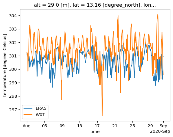
2m temperature at the BCO in Aug-Sep 2020#
We would like to plot the 2m air temperature at one location, the BCO, in August and September 2020. For this rather short time period, we would like to work with the hourly data. Therefore, we need to specify the time hierarchy when addressing the data in the catalog.
era5 = cat.HERA5(time="PT1H").to_dask().pipe(egh.attach_coords)
/home/runner/miniconda3/envs/orcestra_book/lib/python3.12/site-packages/intake_xarray/xzarr.py:44: FutureWarning: In a future version of xarray the default value for compat will change from compat='no_conflicts' to compat='override'. This is likely to lead to different results when combining overlapping variables with the same name. To opt in to new defaults and get rid of these warnings now use `set_options(use_new_combine_kwarg_defaults=True) or set compat explicitly.
  self._ds = xr.open_mfdataset(self.urlpath, **kw)
/home/runner/miniconda3/envs/orcestra_book/lib/python3.12/site-packages/intake_xarray/base.py:21: FutureWarning: The return type of `Dataset.dims` will be changed to return a set of dimension names in future, in order to be more consistent with `DataArray.dims`. To access a mapping from dimension names to lengths, please use `Dataset.sizes`.
  'dims': dict(self._ds.dims),
Intake v2
The recent Intake v2 libraries do not support parameters!
Make sure you constrain the Intake version to intake<2 and intake-xarray<2 during installation.
Next, we want to see how temperature readings at BCO (WXT) compare with the ERA5 reanalysis.
We select the cell index that is the nearest neighbor to the BCO location using healpix.ang2pix().
wxt = cat.BCO.surfacemet_wxt_v1.to_dask()
i_bco = hp.ang2pix(egh.get_nside(era5), wxt.lon, wxt.lat, nest=egh.get_nest(era5), lonlat=True)
/home/runner/miniconda3/envs/orcestra_book/lib/python3.12/site-packages/intake_xarray/base.py:21: FutureWarning: The return type of `Dataset.dims` will be changed to return a set of dimension names in future, in order to be more consistent with `DataArray.dims`. To access a mapping from dimension names to lengths, please use `Dataset.sizes`.
  'dims': dict(self._ds.dims),
Now, we can plot the time series by selecting the respective cell as well as a time range:
era5["2t"].isel(cell=i_bco).sel(time="2020-08").plot(label="ERA5")
(wxt["T"].sel(time="2020-08").resample(time="1h").mean() + 273.15).plot(label="WXT")
plt.legend();
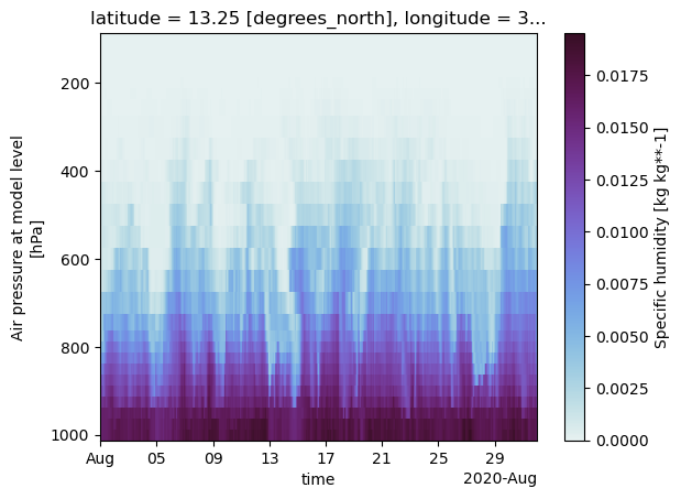
Evolution of the moisture field at BCO#
Next, we extend our analysis and use a 3d variable to plot a time-height diagramm of moisture.
Again, we select the BCO cell, a time range and now also a range in height level where we leave out the upper most layers (<100hPa) as we are interested in the troposphere only.
era5["q"].sel(
    cell=i_bco,
    time="2020-08",
    level=slice(100, 1000),
).plot(
    x="time",
    yincrease=False,
    cmap="cmo.dense",
    vmin=0,
)
<matplotlib.collections.QuadMesh at 0x7f9994f34200>
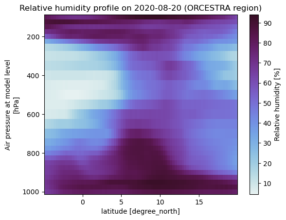
Select ORCESTRA region#
We want to see how the RH profile changes with latitude when averaged over the ORCESTRA campaign region on the 20th of August 2020. The easygems package provides the the isel_extent function which takes a lat/lon extent ([W, E, S, N]) as input and returns the corresponding indices of the global HEALPix grid. These indices can then be used to select the region of interest.
is_orcestra = egh.isel_extent(era5, [-60, -10, -5, 20])

fig, ax = plt.subplots()
era5["r"].sel(
    cell=is_orcestra,
    time="2020-08-20",
    level=slice(100, 1000),
).mean(
    "time"
).groupby(
    era5.lat.sel(cell=is_orcestra)
).mean().plot(
    x="lat",
    yincrease=False,
    cmap="cmo.dense",
    ax=ax,
)
ax.set_title("Relative humidity profile on 2020-08-20 (ORCESTRA region)")
Text(0.5, 1.0, 'Relative humidity profile on 2020-08-20 (ORCESTRA region)')
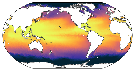
A snapshot of global SST#
egh.healpix_show(
    era5["sst"].sel(time="2020-08-01T12:00:00", method="nearest"),
    nest=egh.get_nest(era5),
    vmin=273,
    vmax=303,
    cmap="cmo.thermal",
)
<matplotlib.image.AxesImage at 0x7f9994f369c0>
/home/runner/miniconda3/envs/orcestra_book/lib/python3.12/site-packages/cartopy/io/__init__.py:242: DownloadWarning: Downloading: https://naturalearth.s3.amazonaws.com/110m_physical/ne_110m_coastline.zip
  warnings.warn(f'Downloading: {url}', DownloadWarning)
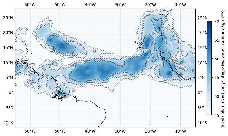
Plotting the Atlantic basin only#
In real-life analyses it is often necessary to constrain a plot to certain regions.
The function easygems.healpix_show() allows to plot two-dimensional data onto a cartopy GeoAxis with arbitrary projection and extent.
Here, we plot contour lines of the integrated water-vapor (IWV), which plays a crucial role in the flight planning of PERCUSION.
era5 = cat.HERA5(time="PT1H").to_dask().pipe(egh.attach_coords)
iwv = era5["tcwv"].sel(time="2020-08", method="nearest")

fig, ax = plt.subplots(figsize=(10, 6), subplot_kw={"projection": ccrs.PlateCarree()})
ax.gridlines(draw_labels=True, dms=True, x_inline=False, y_inline=False, alpha=0.25)
ax.set_extent([-65, -5, -10, 25])
ax.coastlines(lw=0.8)

im = egh.healpix_show(iwv, cmap="Blues", vmin=45, vmax=70)
fig.colorbar(im, label=f"{iwv.long_name} / {iwv.units}", shrink=0.7)

clines = egh.healpix_contour(iwv, levels=[45, 50, 55], colors="k", linewidths=1, alpha=0.5)
ax.clabel(clines, inline=True, fontsize=10, colors="k", fmt="%d");
/home/runner/miniconda3/envs/orcestra_book/lib/python3.12/site-packages/intake_xarray/xzarr.py:44: FutureWarning: In a future version of xarray the default value for compat will change from compat='no_conflicts' to compat='override'. This is likely to lead to different results when combining overlapping variables with the same name. To opt in to new defaults and get rid of these warnings now use `set_options(use_new_combine_kwarg_defaults=True) or set compat explicitly.
  self._ds = xr.open_mfdataset(self.urlpath, **kw)
/home/runner/miniconda3/envs/orcestra_book/lib/python3.12/site-packages/intake_xarray/base.py:21: FutureWarning: The return type of `Dataset.dims` will be changed to return a set of dimension names in future, in order to be more consistent with `DataArray.dims`. To access a mapping from dimension names to lengths, please use `Dataset.sizes`.
  'dims': dict(self._ds.dims),
Further reading#
The HEALPix grid: A short intro