IFS forecasts#
The ECMWF kindly provides their IFS forecast data on a public server. We have started to automatically download the individual GRIB data, create a unified dataset, and remap it onto the HEALPix grid. This dataset, which we call HIFS, is accessible through the internal TCO catalog and can be read and used by everyone. HIFS provides data at different initial dates (twice a day) starting in February 2024. This notebook shows the access to the data and some basic usage examples.
Tip
The access and usage of the data is the same as for HERA5, which you might want to check out too.
Loading the data from the catalog#
First, let’s import all packages that are required to run the full notebook.
import intake
import healpix as hp
import cmocean
import numpy as np
import xarray as xr

import cartopy.crs as ccrs
import cartopy.feature as cf
import matplotlib.pyplot as plt

import easygems.healpix as egh
Now we can open the catalog and select the HEALPix-ified IFS forecast HIFS.
cat = intake.open_catalog("https://tcodata.mpimet.mpg.de/internal.yaml")
ds = cat.HIFS(datetime="2024-04-01").to_dask().pipe(egh.attach_coords)
ds
/home/runner/miniconda3/envs/orcestra_book/lib/python3.12/site-packages/intake_xarray/base.py:21: FutureWarning: The return type of `Dataset.dims` will be changed to return a set of dimension names in future, in order to be more consistent with `DataArray.dims`. To access a mapping from dimension names to lengths, please use `Dataset.sizes`.
  'dims': dict(self._ds.dims),
<xarray.Dataset> Size: 7GB
Dimensions:  (time: 64, cell: 196608, level: 13)
Coordinates:
  * time     (time) datetime64[ns] 512B 2024-04-01T03:00:00 ... 2024-04-11
  * cell     (cell) int64 2MB 0 1 2 3 4 5 ... 196603 196604 196605 196606 196607
    lat      (cell) float64 2MB 0.2984 0.5968 0.5968 ... -0.5968 -0.5968 -0.2984
    lon      (cell) float64 2MB 45.0 45.35 44.65 45.0 ... 315.4 314.6 315.0
  * level    (level) int64 104B 50 100 150 200 250 300 ... 600 700 850 925 1000
    crs      int64 8B 0
Data variables: (12/39)
    100u     (time, cell) float32 50MB dask.array<chunksize=(6, 16384), meta=np.ndarray>
    100v     (time, cell) float32 50MB dask.array<chunksize=(6, 16384), meta=np.ndarray>
    10u      (time, cell) float32 50MB dask.array<chunksize=(6, 16384), meta=np.ndarray>
    10v      (time, cell) float32 50MB dask.array<chunksize=(6, 16384), meta=np.ndarray>
    2d       (time, cell) float32 50MB dask.array<chunksize=(6, 16384), meta=np.ndarray>
    2t       (time, cell) float32 50MB dask.array<chunksize=(6, 16384), meta=np.ndarray>
    ...       ...
    tp       (time, cell) float32 50MB dask.array<chunksize=(6, 16384), meta=np.ndarray>
    ttr      (time, cell) float32 50MB dask.array<chunksize=(6, 16384), meta=np.ndarray>
    u        (time, level, cell) float32 654MB dask.array<chunksize=(6, 1, 16384), meta=np.ndarray>
    v        (time, level, cell) float32 654MB dask.array<chunksize=(6, 1, 16384), meta=np.ndarray>
    vo       (time, level, cell) float32 654MB dask.array<chunksize=(6, 1, 16384), meta=np.ndarray>
w (time, level, cell) float32 654MB dask.array<chunksize=(6, 1, 16384), meta=np.ndarray>- time: 64
- cell: 196608
- level: 13
- time(time)datetime64[ns]2024-04-01T03:00:00 ... 2024-04-11
- axis :
- T
array(['2024-04-01T03:00:00.000000000', '2024-04-01T06:00:00.000000000', '2024-04-01T09:00:00.000000000', '2024-04-01T12:00:00.000000000', '2024-04-01T15:00:00.000000000', '2024-04-01T18:00:00.000000000', '2024-04-01T21:00:00.000000000', '2024-04-02T00:00:00.000000000', '2024-04-02T03:00:00.000000000', '2024-04-02T06:00:00.000000000', '2024-04-02T09:00:00.000000000', '2024-04-02T12:00:00.000000000', '2024-04-02T15:00:00.000000000', '2024-04-02T18:00:00.000000000', '2024-04-02T21:00:00.000000000', '2024-04-03T00:00:00.000000000', '2024-04-03T03:00:00.000000000', '2024-04-03T06:00:00.000000000', '2024-04-03T09:00:00.000000000', '2024-04-03T12:00:00.000000000', '2024-04-03T15:00:00.000000000', '2024-04-03T18:00:00.000000000', '2024-04-03T21:00:00.000000000', '2024-04-04T00:00:00.000000000', '2024-04-04T03:00:00.000000000', '2024-04-04T06:00:00.000000000', '2024-04-04T09:00:00.000000000', '2024-04-04T12:00:00.000000000', '2024-04-04T15:00:00.000000000', '2024-04-04T18:00:00.000000000', '2024-04-04T21:00:00.000000000', '2024-04-05T00:00:00.000000000', '2024-04-05T03:00:00.000000000', '2024-04-05T06:00:00.000000000', '2024-04-05T09:00:00.000000000', '2024-04-05T12:00:00.000000000', '2024-04-05T15:00:00.000000000', '2024-04-05T18:00:00.000000000', '2024-04-05T21:00:00.000000000', '2024-04-06T00:00:00.000000000', '2024-04-06T03:00:00.000000000', '2024-04-06T06:00:00.000000000', '2024-04-06T09:00:00.000000000', '2024-04-06T12:00:00.000000000', '2024-04-06T15:00:00.000000000', '2024-04-06T18:00:00.000000000', '2024-04-06T21:00:00.000000000', '2024-04-07T00:00:00.000000000', '2024-04-07T06:00:00.000000000', '2024-04-07T12:00:00.000000000', '2024-04-07T18:00:00.000000000', '2024-04-08T00:00:00.000000000', '2024-04-08T06:00:00.000000000', '2024-04-08T12:00:00.000000000', '2024-04-08T18:00:00.000000000', '2024-04-09T00:00:00.000000000', '2024-04-09T06:00:00.000000000', '2024-04-09T12:00:00.000000000', '2024-04-09T18:00:00.000000000', '2024-04-10T00:00:00.000000000', '2024-04-10T06:00:00.000000000', '2024-04-10T12:00:00.000000000', '2024-04-10T18:00:00.000000000', '2024-04-11T00:00:00.000000000'], dtype='datetime64[ns]') - cell(cell)int640 1 2 3 ... 196605 196606 196607
- standard_name :
- healpix_index
array([ 0, 1, 2, ..., 196605, 196606, 196607], shape=(196608,))
- lat(cell)float640.2984 0.5968 ... -0.5968 -0.2984
- units :
- degree_north
- standard_name :
- latitude
- axis :
- Y
array([ 0.29841687, 0.59684183, 0.59684183, ..., -0.59684183, -0.59684183, -0.29841687], shape=(196608,)) - lon(cell)float6445.0 45.35 44.65 ... 314.6 315.0
- units :
- degree_east
- standard_name :
- longitude
- axis :
- X
array([ 45. , 45.3515625, 44.6484375, ..., 315.3515625, 314.6484375, 315. ], shape=(196608,)) - level(level)int6450 100 150 200 ... 700 850 925 1000
- axis :
- Z
- long_name :
- Air pressure at model level
- positive :
- down
- standard_name :
- air_pressure
- units :
- hPa
array([ 50, 100, 150, 200, 250, 300, 400, 500, 600, 700, 850, 925, 1000]) - crs()int640
- grid_mapping_name :
- healpix
- refinement_level :
- 7
- indexing_scheme :
- nested
array(0)
- 100u(time, cell)float32dask.array<chunksize=(6, 16384), meta=np.ndarray>
- levtype :
- heightAboveGround
- long_name :
- 100 metre U wind component
- standard_name :
- eastward_wind
- type :
- forecast
- units :
- m s**-1
Array Chunk Bytes 48.00 MiB 384.00 kiB Shape (64, 196608) (6, 16384) Dask graph 132 chunks in 2 graph layers Data type float32 numpy.ndarray - 100v(time, cell)float32dask.array<chunksize=(6, 16384), meta=np.ndarray>
- levtype :
- heightAboveGround
- long_name :
- 100 metre V wind component
- standard_name :
- northward_wind
- type :
- forecast
- units :
- m s**-1
Array Chunk Bytes 48.00 MiB 384.00 kiB Shape (64, 196608) (6, 16384) Dask graph 132 chunks in 2 graph layers Data type float32 numpy.ndarray - 10u(time, cell)float32dask.array<chunksize=(6, 16384), meta=np.ndarray>
- levtype :
- heightAboveGround
- long_name :
- 10 metre U wind component
- standard_name :
- eastward_wind
- type :
- forecast
- units :
- m s**-1
Array Chunk Bytes 48.00 MiB 384.00 kiB Shape (64, 196608) (6, 16384) Dask graph 132 chunks in 2 graph layers Data type float32 numpy.ndarray - 10v(time, cell)float32dask.array<chunksize=(6, 16384), meta=np.ndarray>
- levtype :
- heightAboveGround
- long_name :
- 10 metre V wind component
- standard_name :
- northward_wind
- type :
- forecast
- units :
- m s**-1
Array Chunk Bytes 48.00 MiB 384.00 kiB Shape (64, 196608) (6, 16384) Dask graph 132 chunks in 2 graph layers Data type float32 numpy.ndarray - 2d(time, cell)float32dask.array<chunksize=(6, 16384), meta=np.ndarray>
- levtype :
- heightAboveGround
- long_name :
- 2 metre dewpoint temperature
- standard_name :
- type :
- forecast
- units :
- K
Array Chunk Bytes 48.00 MiB 384.00 kiB Shape (64, 196608) (6, 16384) Dask graph 132 chunks in 2 graph layers Data type float32 numpy.ndarray - 2t(time, cell)float32dask.array<chunksize=(6, 16384), meta=np.ndarray>
- levtype :
- heightAboveGround
- long_name :
- 2 metre temperature
- standard_name :
- air_temperature
- type :
- forecast
- units :
- K
Array Chunk Bytes 48.00 MiB 384.00 kiB Shape (64, 196608) (6, 16384) Dask graph 132 chunks in 2 graph layers Data type float32 numpy.ndarray - asn(time, cell)float32dask.array<chunksize=(6, 16384), meta=np.ndarray>
- levtype :
- surface
- long_name :
- Snow albedo
- standard_name :
- type :
- forecast
- units :
- (0 - 1)
Array Chunk Bytes 48.00 MiB 384.00 kiB Shape (64, 196608) (6, 16384) Dask graph 132 chunks in 2 graph layers Data type float32 numpy.ndarray - cape(time, cell)float32dask.array<chunksize=(6, 16384), meta=np.ndarray>
- levtype :
- entireAtmosphere
- long_name :
- Convective available potential energy
- standard_name :
- type :
- forecast
- units :
- J kg**-1
Array Chunk Bytes 48.00 MiB 384.00 kiB Shape (64, 196608) (6, 16384) Dask graph 132 chunks in 2 graph layers Data type float32 numpy.ndarray - d(time, level, cell)float32dask.array<chunksize=(6, 1, 16384), meta=np.ndarray>
- levtype :
- isobaricInhPa
- long_name :
- Divergence
- standard_name :
- divergence_of_wind
- type :
- forecast
- units :
- s**-1
Array Chunk Bytes 624.00 MiB 384.00 kiB Shape (64, 13, 196608) (6, 1, 16384) Dask graph 1716 chunks in 2 graph layers Data type float32 numpy.ndarray - gh(time, level, cell)float32dask.array<chunksize=(6, 1, 16384), meta=np.ndarray>
- levtype :
- isobaricInhPa
- long_name :
- Geopotential height
- standard_name :
- geopotential_height
- type :
- forecast
- units :
- gpm
Array Chunk Bytes 624.00 MiB 384.00 kiB Shape (64, 13, 196608) (6, 1, 16384) Dask graph 1716 chunks in 2 graph layers Data type float32 numpy.ndarray - lsm(time, cell)float32dask.array<chunksize=(6, 16384), meta=np.ndarray>
- levtype :
- surface
- long_name :
- Land-sea mask
- standard_name :
- land_binary_mask
- type :
- forecast
- units :
- (0 - 1)
Array Chunk Bytes 48.00 MiB 384.00 kiB Shape (64, 196608) (6, 16384) Dask graph 132 chunks in 2 graph layers Data type float32 numpy.ndarray - mn2t6(time, cell)float32dask.array<chunksize=(6, 16384), meta=np.ndarray>
- levtype :
- heightAboveGround
- long_name :
- Minimum temperature at 2 metres in the last 6 hours
- standard_name :
- air_temperature
- type :
- forecast
- units :
- K
Array Chunk Bytes 48.00 MiB 384.00 kiB Shape (64, 196608) (6, 16384) Dask graph 132 chunks in 2 graph layers Data type float32 numpy.ndarray - msl(time, cell)float32dask.array<chunksize=(6, 16384), meta=np.ndarray>
- levtype :
- meanSea
- long_name :
- Mean sea level pressure
- standard_name :
- air_pressure_at_mean_sea_level
- type :
- forecast
- units :
- Pa
Array Chunk Bytes 48.00 MiB 384.00 kiB Shape (64, 196608) (6, 16384) Dask graph 132 chunks in 2 graph layers Data type float32 numpy.ndarray - mx2t6(time, cell)float32dask.array<chunksize=(6, 16384), meta=np.ndarray>
- levtype :
- heightAboveGround
- long_name :
- Maximum temperature at 2 metres in the last 6 hours
- standard_name :
- air_temperature
- type :
- forecast
- units :
- K
Array Chunk Bytes 48.00 MiB 384.00 kiB Shape (64, 196608) (6, 16384) Dask graph 132 chunks in 2 graph layers Data type float32 numpy.ndarray - q(time, level, cell)float32dask.array<chunksize=(6, 1, 16384), meta=np.ndarray>
- levtype :
- isobaricInhPa
- long_name :
- Specific humidity
- standard_name :
- specific_humidity
- type :
- forecast
- units :
- kg kg**-1
Array Chunk Bytes 624.00 MiB 384.00 kiB Shape (64, 13, 196608) (6, 1, 16384) Dask graph 1716 chunks in 2 graph layers Data type float32 numpy.ndarray - r(time, level, cell)float32dask.array<chunksize=(6, 1, 16384), meta=np.ndarray>
- levtype :
- isobaricInhPa
- long_name :
- Relative humidity
- standard_name :
- relative_humidity
- type :
- forecast
- units :
- %
Array Chunk Bytes 624.00 MiB 384.00 kiB Shape (64, 13, 196608) (6, 1, 16384) Dask graph 1716 chunks in 2 graph layers Data type float32 numpy.ndarray - ro(time, cell)float32dask.array<chunksize=(6, 16384), meta=np.ndarray>
- levtype :
- surface
- long_name :
- Runoff
- standard_name :
- type :
- forecast
- units :
- m
Array Chunk Bytes 48.00 MiB 384.00 kiB Shape (64, 196608) (6, 16384) Dask graph 132 chunks in 2 graph layers Data type float32 numpy.ndarray - skt(time, cell)float32dask.array<chunksize=(6, 16384), meta=np.ndarray>
- levtype :
- surface
- long_name :
- Skin temperature
- standard_name :
- type :
- forecast
- units :
- K
Array Chunk Bytes 48.00 MiB 384.00 kiB Shape (64, 196608) (6, 16384) Dask graph 132 chunks in 2 graph layers Data type float32 numpy.ndarray - sp(time, cell)float32dask.array<chunksize=(6, 16384), meta=np.ndarray>
- levtype :
- surface
- long_name :
- Surface pressure
- standard_name :
- surface_air_pressure
- type :
- forecast
- units :
- Pa
Array Chunk Bytes 48.00 MiB 384.00 kiB Shape (64, 196608) (6, 16384) Dask graph 132 chunks in 2 graph layers Data type float32 numpy.ndarray - ssr(time, cell)float32dask.array<chunksize=(6, 16384), meta=np.ndarray>
- levtype :
- surface
- long_name :
- Surface net short-wave (solar) radiation
- standard_name :
- surface_net_downward_shortwave_flux
- type :
- forecast
- units :
- J m**-2
Array Chunk Bytes 48.00 MiB 384.00 kiB Shape (64, 196608) (6, 16384) Dask graph 132 chunks in 2 graph layers Data type float32 numpy.ndarray - ssrd(time, cell)float32dask.array<chunksize=(6, 16384), meta=np.ndarray>
- levtype :
- surface
- long_name :
- Surface short-wave (solar) radiation downwards
- standard_name :
- surface_downwelling_shortwave_flux_in_air
- type :
- forecast
- units :
- J m**-2
Array Chunk Bytes 48.00 MiB 384.00 kiB Shape (64, 196608) (6, 16384) Dask graph 132 chunks in 2 graph layers Data type float32 numpy.ndarray - st(time, cell)float32dask.array<chunksize=(6, 16384), meta=np.ndarray>
- levtype :
- depthBelowLandLayer
- long_name :
- Soil temperature
- standard_name :
- type :
- forecast
- units :
- K
Array Chunk Bytes 48.00 MiB 384.00 kiB Shape (64, 196608) (6, 16384) Dask graph 132 chunks in 2 graph layers Data type float32 numpy.ndarray - stl2(time, cell)float32dask.array<chunksize=(6, 16384), meta=np.ndarray>
- levtype :
- depthBelowLandLayer
- long_name :
- Soil temperature level 2
- standard_name :
- type :
- forecast
- units :
- K
Array Chunk Bytes 48.00 MiB 384.00 kiB Shape (64, 196608) (6, 16384) Dask graph 132 chunks in 2 graph layers Data type float32 numpy.ndarray - stl3(time, cell)float32dask.array<chunksize=(6, 16384), meta=np.ndarray>
- levtype :
- depthBelowLandLayer
- long_name :
- Soil temperature level 3
- standard_name :
- type :
- forecast
- units :
- K
Array Chunk Bytes 48.00 MiB 384.00 kiB Shape (64, 196608) (6, 16384) Dask graph 132 chunks in 2 graph layers Data type float32 numpy.ndarray - stl4(time, cell)float32dask.array<chunksize=(6, 16384), meta=np.ndarray>
- levtype :
- depthBelowLandLayer
- long_name :
- Soil temperature level 4
- standard_name :
- type :
- forecast
- units :
- K
Array Chunk Bytes 48.00 MiB 384.00 kiB Shape (64, 196608) (6, 16384) Dask graph 132 chunks in 2 graph layers Data type float32 numpy.ndarray - str(time, cell)float32dask.array<chunksize=(6, 16384), meta=np.ndarray>
- levtype :
- surface
- long_name :
- Surface net long-wave (thermal) radiation
- standard_name :
- surface_net_upward_longwave_flux
- type :
- forecast
- units :
- J m**-2
Array Chunk Bytes 48.00 MiB 384.00 kiB Shape (64, 196608) (6, 16384) Dask graph 132 chunks in 2 graph layers Data type float32 numpy.ndarray - strd(time, cell)float32dask.array<chunksize=(6, 16384), meta=np.ndarray>
- levtype :
- surface
- long_name :
- Surface long-wave (thermal) radiation downwards
- standard_name :
- type :
- forecast
- units :
- J m**-2
Array Chunk Bytes 48.00 MiB 384.00 kiB Shape (64, 196608) (6, 16384) Dask graph 132 chunks in 2 graph layers Data type float32 numpy.ndarray - swvl1(time, cell)float32dask.array<chunksize=(6, 16384), meta=np.ndarray>
- levtype :
- depthBelowLandLayer
- long_name :
- Volumetric soil water layer 1
- standard_name :
- type :
- forecast
- units :
- m**3 m**-3
Array Chunk Bytes 48.00 MiB 384.00 kiB Shape (64, 196608) (6, 16384) Dask graph 132 chunks in 2 graph layers Data type float32 numpy.ndarray - swvl2(time, cell)float32dask.array<chunksize=(6, 16384), meta=np.ndarray>
- levtype :
- depthBelowLandLayer
- long_name :
- Volumetric soil water layer 2
- standard_name :
- type :
- forecast
- units :
- m**3 m**-3
Array Chunk Bytes 48.00 MiB 384.00 kiB Shape (64, 196608) (6, 16384) Dask graph 132 chunks in 2 graph layers Data type float32 numpy.ndarray - swvl3(time, cell)float32dask.array<chunksize=(6, 16384), meta=np.ndarray>
- levtype :
- depthBelowLandLayer
- long_name :
- Volumetric soil water layer 3
- standard_name :
- type :
- forecast
- units :
- m**3 m**-3
Array Chunk Bytes 48.00 MiB 384.00 kiB Shape (64, 196608) (6, 16384) Dask graph 132 chunks in 2 graph layers Data type float32 numpy.ndarray - swvl4(time, cell)float32dask.array<chunksize=(6, 16384), meta=np.ndarray>
- levtype :
- depthBelowLandLayer
- long_name :
- Volumetric soil water layer 4
- standard_name :
- type :
- forecast
- units :
- m**3 m**-3
Array Chunk Bytes 48.00 MiB 384.00 kiB Shape (64, 196608) (6, 16384) Dask graph 132 chunks in 2 graph layers Data type float32 numpy.ndarray - t(time, level, cell)float32dask.array<chunksize=(6, 1, 16384), meta=np.ndarray>
- levtype :
- isobaricInhPa
- long_name :
- Temperature
- standard_name :
- air_temperature
- type :
- forecast
- units :
- K
Array Chunk Bytes 624.00 MiB 384.00 kiB Shape (64, 13, 196608) (6, 1, 16384) Dask graph 1716 chunks in 2 graph layers Data type float32 numpy.ndarray - tcwv(time, cell)float32dask.array<chunksize=(6, 16384), meta=np.ndarray>
- levtype :
- entireAtmosphere
- long_name :
- Total column vertically-integrated water vapour
- standard_name :
- lwe_thickness_of_atmosphere_mass_content_of_water_vapor
- type :
- forecast
- units :
- kg m**-2
Array Chunk Bytes 48.00 MiB 384.00 kiB Shape (64, 196608) (6, 16384) Dask graph 132 chunks in 2 graph layers Data type float32 numpy.ndarray - tp(time, cell)float32dask.array<chunksize=(6, 16384), meta=np.ndarray>
- levtype :
- surface
- long_name :
- Total precipitation
- standard_name :
- type :
- forecast
- units :
- m
Array Chunk Bytes 48.00 MiB 384.00 kiB Shape (64, 196608) (6, 16384) Dask graph 132 chunks in 2 graph layers Data type float32 numpy.ndarray - ttr(time, cell)float32dask.array<chunksize=(6, 16384), meta=np.ndarray>
- levtype :
- nominalTop
- long_name :
- Top net long-wave (thermal) radiation
- standard_name :
- toa_outgoing_longwave_flux
- type :
- forecast
- units :
- J m**-2
Array Chunk Bytes 48.00 MiB 384.00 kiB Shape (64, 196608) (6, 16384) Dask graph 132 chunks in 2 graph layers Data type float32 numpy.ndarray - u(time, level, cell)float32dask.array<chunksize=(6, 1, 16384), meta=np.ndarray>
- levtype :
- isobaricInhPa
- long_name :
- U component of wind
- standard_name :
- eastward_wind
- type :
- forecast
- units :
- m s**-1
Array Chunk Bytes 624.00 MiB 384.00 kiB Shape (64, 13, 196608) (6, 1, 16384) Dask graph 1716 chunks in 2 graph layers Data type float32 numpy.ndarray - v(time, level, cell)float32dask.array<chunksize=(6, 1, 16384), meta=np.ndarray>
- levtype :
- isobaricInhPa
- long_name :
- V component of wind
- standard_name :
- northward_wind
- type :
- forecast
- units :
- m s**-1
Array Chunk Bytes 624.00 MiB 384.00 kiB Shape (64, 13, 196608) (6, 1, 16384) Dask graph 1716 chunks in 2 graph layers Data type float32 numpy.ndarray - vo(time, level, cell)float32dask.array<chunksize=(6, 1, 16384), meta=np.ndarray>
- levtype :
- isobaricInhPa
- long_name :
- Vorticity (relative)
- standard_name :
- atmosphere_relative_vorticity
- type :
- forecast
- units :
- s**-1
Array Chunk Bytes 624.00 MiB 384.00 kiB Shape (64, 13, 196608) (6, 1, 16384) Dask graph 1716 chunks in 2 graph layers Data type float32 numpy.ndarray - w(time, level, cell)float32dask.array<chunksize=(6, 1, 16384), meta=np.ndarray>
- levtype :
- isobaricInhPa
- long_name :
- Vertical velocity
- standard_name :
- lagrangian_tendency_of_air_pressure
- type :
- forecast
- units :
- Pa s**-1
Array Chunk Bytes 624.00 MiB 384.00 kiB Shape (64, 13, 196608) (6, 1, 16384) Dask graph 1716 chunks in 2 graph layers Data type float32 numpy.ndarray
Plotting examples#
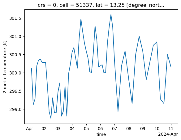
2m temperature at the BCO#
We would like to plot the 2m air temperature at one location, the BCO.
ds = cat.HIFS(datetime="2024-04-01").to_dask().pipe(egh.attach_coords)

i_bco = hp.ang2pix(
    egh.get_nside(ds),
    -59.42875, # longitude at BCO
    13.16264, # latitude at BCO
    nest=egh.get_nest(ds),
    lonlat=True,
)

ds["2t"].sel(cell=i_bco).plot()
/home/runner/miniconda3/envs/orcestra_book/lib/python3.12/site-packages/intake_xarray/base.py:21: FutureWarning: The return type of `Dataset.dims` will be changed to return a set of dimension names in future, in order to be more consistent with `DataArray.dims`. To access a mapping from dimension names to lengths, please use `Dataset.sizes`.
  'dims': dict(self._ds.dims),
[<matplotlib.lines.Line2D at 0x7f8a149ce330>]
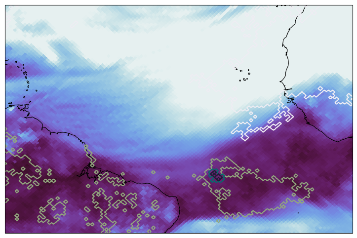
Select ORCESTRA region#
Plotting the forecasted total column water vapor and precipitation contours over the campaign domain.
Plotting maps
You may want to check out this tutorial on ways to plot geospatial data.
fig, ax = plt.subplots(figsize=(10, 6), subplot_kw={"projection": ccrs.PlateCarree()})
ax.set_extent([-65, -5, -10, 25])
ax.coastlines(lw=0.8)
egh.healpix_show(
    ds["tcwv"].sel(time="2024-04-05 12:00"),
    cmap="cmo.dense",
    vmin=25,
    vmax=65,
)

egh.healpix_contour(
    ds["tp"].sel(time="2024-04-05 12:00"),
    cmap="cmo.rain",
    vmin=0.,
    vmax=0.15,
    levels=5,
)
<cartopy.mpl.contour.GeoContourSet at 0x7f8a2445bbc0>